PQStat - Baza Wiedzy

Group heterogeneity

Examination of group heterogeneity

We can compare groups by choosing as overall effect: fixed effect, random effect – separate $T^2$ or random effect – pooled $T^2$ , where $T^2$ is the variance of the observed effects.

Fixed effect is chosen when we assume that studies within each group share one common true (i.e., population) effect.
Random effect (separate $T^2$ ) is chosen when we assume that the studies within each group represent slightly different populations, and the groups differ in variance between studies.
Random effect (pooled $T^2$ ) is chosen when we assume that the studies within each group represent slightly different populations, but the variance between studies is the same, regardless of the group to which they belong.

The main goal is to compare groups, that is, to determine whether the groups being compared differ in their true (i.e., population) overall effect. In practice, this is to test whether the variance of group overall effects is zero, i.e., to test the heterogeneity of the groups. For a description and interpretation of the results of heterogeneity analysis, see chapter Heterogeneity testing, except that in the case of group comparisons, heterogeneity refers to the compound effects of the groups being compared, not the individual studies, and the outcome depends on the overall effect chosen.

Hypotheses:

$\begin{array}{cl} \mathcal{H}_0: & \tau^2 = 0,\\ \mathcal{H}_1: & \tau^2 \ne 0, \end{array}$

where:

$\tau^2$ – is the variance of the true (population) summary effects of the groups being compared.

The p value, designated on the basis of the test statistic, is compared with the significance level $\alpha$ :

$\begin{array}{ccl} $ if $ p \le \alpha & \Longrightarrow & $ reject $ \mathcal{H}_0 $ and accept $ \mathcal{H}_1, \\ $ if $ p > \alpha & \Longrightarrow & $ there is no reason to reject $ \mathcal{H}_0. \\ \end{array}$

If the result is statistically significant (a score of Q-statistic, $I^2$ coefficient or $H^2$ coefficient), this is a strong suggestion to drop the overall summary of the groups being compared.

Examining heterogeneity in groups

An additional option of the analysis is the possibility to analyze each group separately for heterogeneity, as described in Heterogeneity testing. The results obtained (in particular, the variance $T^2$ ) make it easier to decide how to compare the groups, i.e., whether to choose a random effect (separate $T^2$ ) or a random effect (pooled $T^2$ ).

Joint summary of the groups

In a situation where, based on the results of the group comparison, the differences obtained between the overall effects of the groups are small and insignificant, a joint summary of the groups can be performed. The summation is done in correction for the division into the indicated groups. For example, if we split the study based on the different conditions of the experiment conducted, then the joint summary will be done in correction for the different conditions of the experiment. The result of joint summation (overall efect of both grous) depends on the observed differences (on the variation between studies and between groups) i.e. on the choice of ovearall effect (whether it is fixed or random (separate $T^2$ ) or random (pooled $T^2$ )).

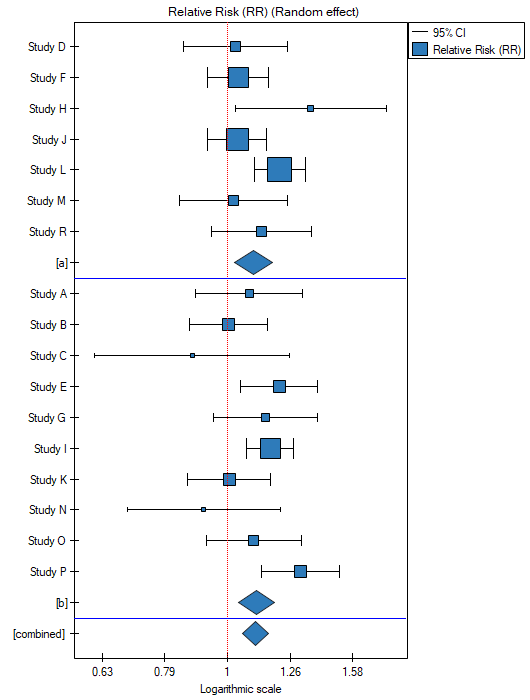
A good illustration of the joint (ovearall) summary of the groups in the meta-analysis is a forest plot showing the results of each study with each group's summary and the joint summary of the groups.

ANOVA comparison

ANOVA comparison is an additional option for comparing groups. It is a slightly different method of comparison than comparison by testing heterogeneity of groups (based on a different mathematical model). Both methods, however, give overlapping results as to the comparison of groups. In case of comparison of groups by ANOVA method the observed variance is broken down into between-group variance and within-group variance. The within-group variance is then broken down into the variance of each group separately. As a result, the following $Q$ statistics are determined:

The $Q$ statistic (group 1) – examines that part of the total variance that relates to group one, i.e., the variance between studies located within group one,
The $Q$ statistic (group 2) – examines that part of the total variance that relates to the second group, i.e. the variance between studies within the second group,
…
The $Q$ statistic (group g) – examines that part of the total variance that relates to the last group, i.e., the variance between studies within the last group,
The $Q$ statistic (within groups) = $Q$ (group 1) + $Q$ (group 2) + … + $Q$ (group g) - examines that part of the total variance that relates to the inside of the individual groups, i.e., the variance of the within-group tests,
The $Q$ statistic (between groups) - examines that part of the total variance that relates to differences between groups, i.e., the between-group variance (same result as examining the heterogeneity of groups) ,
The $Q$ statistic (total) - examines the variance between all studies.

Each of the above $Q$ statistics has a chi-square distribution with the appropriate number of degrees of freedom.

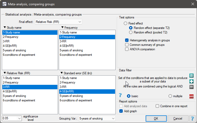
The window with settings of group comparison for meta-analysis is opened via menu: Advanced Statistics→Meta-analysis→Meta-analysis, comparing groups.

EXAMPLE (MetaAnalysisRR.pqs file)

The risk of disease X was examined for smokers and non-smokers. A meta-analysis was conducted to determine whether smoking duration affects the onset of disease X. A thorough review of the literature on this topic was carried out, and 17 studies were identified that had a description of the relative risk and its error (i.e. the precision of the study). Because the studies involved different smoking times, 3 groups of studies were identified:

(1) studies on people who have been smoking for more than 10 years,

(2) studies on people who have been smoking for 5 to 10 years,

(3) studies on people who have been smoking for less than 5 years.

In addition, a subdivision was made between the two different conditions of the studies (different inclusion/exclusion criteria of subjects). Data were prepared for meta-analysis and stored in a file.

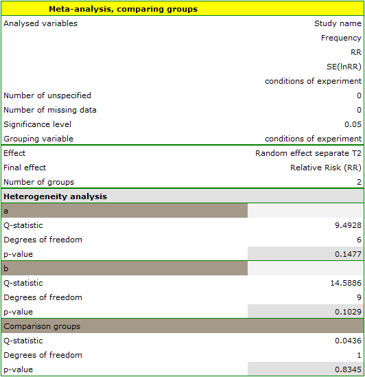
The purpose of conducting the meta-analysis was to compare age groups. In addition, it was examined whether the different conditions of the experiment translated into differences in the relative risk obtained.

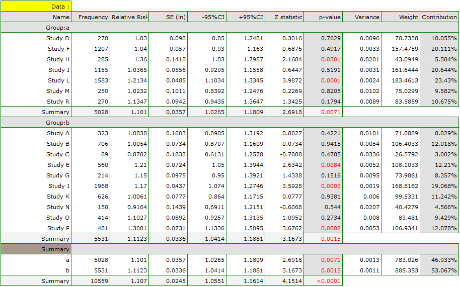
Because the papers included in the meta-analysis were from different locations and included slightly different populations, the summary was made by selecting random effect (separate T2). As the final effect, relative risk was selected and the results were presented on a forest plot.

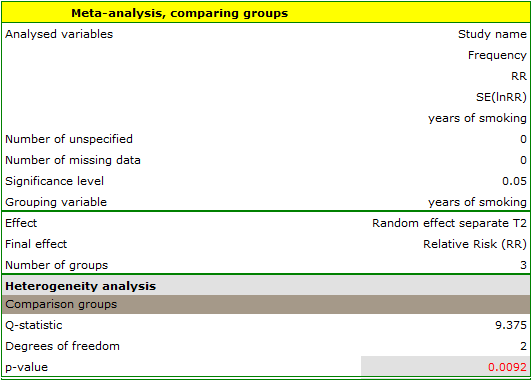
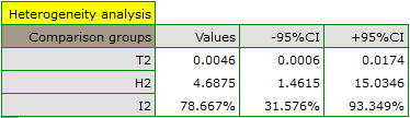
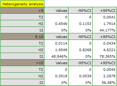
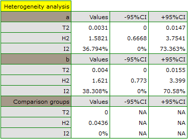
The groups are statistically significantly different (p=0.0092), which we observe not only based on the test of heterogeneity, but also on the coefficient of H2 (the coefficient along with the confidence interval is above the value of one) and I2 (78 is high heterogeneity). Therefore, the collected papers will not be summarized by a overall effect but only by a separate summary of each group.

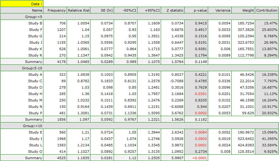
The forest plot also shows a summary of each group and does not contain a joint summary of the groups.

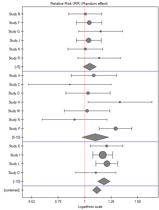
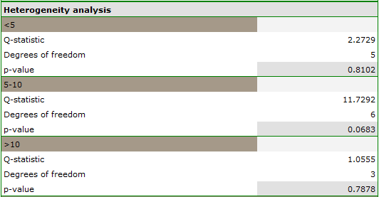
In addition, homogeneity within each group was checked to ascertain the feasibility of summarizing them separately.

In contrast, the results of the comparison concerning the different study conditions indicate that there is no significant effect of these conditions on the overall effect. In this case, it is possible to calculate a joint overall effect when correcting for the different test conditions, i.e., a joint summary of the two groups.

PQStat - Baza Wiedzy

Narzędzia użytkownika

Narzędzia witryny

Pasek boczny

Group heterogeneity

Narzędzia strony