PQStat - Baza Wiedzy

Heterogeneity testing

It is difficult to expect every study to end up with exactly the same effect size. Naturally, the results obtained in different papers will be somewhat different. The study of heterogeneity is intended to determine to what extent emerging differences between the results obtained in different papers affect the overall effect constructed in the meta-analysis. The overall effect summarizes well the results obtained in the different papers if the differences between the different effects are natural i.e. not large. Large differences in observed effects may indicate heterogeneity of studies and the need to separate more homogeneous subgroups, e.g., divide the collected papers into several subgroups with respect to an additional factor. For example: a given drug has a different effect on younger and older people, so in studies based on data from mainly young people, the effect may differ significantly from studies conducted on older people. Dividing the collected papers into more homogenous subgroups will allow for a good estimation of the overall effect for each of these subgroups separately.

Heterogeneity testing is designed to check whether the variability between studies is equal to zero.

Hypotheses:

$\begin{array}{cl} \mathcal{H}_0: & \tau^2 = 0,\\ \mathcal{H}_1: & \tau^2 \ne 0, \end{array}$

where:

$\tau^2$ – is the variance of the true (population) effects of each study.

The test statistic is of the form:

$\begin{displaymath} Q=T^2W+k-1 \end{displaymath}$

where:

$T^2$ – is the variance of the observed effects,

$W$ – a factor calculated from the weights assigned to each study,

$k$ – number of studies.

The statistic has asymptotically (for large sample) chi-squared with the degrees of freedom calculated by the formula: $df=k-1$ .

The p value, designated on the basis of the test statistic, is compared with the significance level $\alpha$ :

$\begin{array}{ccl} $ if $ p \le \alpha & \Longrightarrow & $ reject $ \mathcal{H}_0 $ and accept $ \mathcal{H}_1, \\ $ if $ p > \alpha & \Longrightarrow & $ there is no reason to reject $ \mathcal{H}_0. \\ \end{array}$

Note

If the result is statistically significant – this is a strong suggestion to abandon the overall summary of all collected studies.
If the result obtained is not statistically significant – we can summarize the study with the overall effect. At the same time, it is suggested to summarize with a random effect – according to the following explanation.

Rationale for choosing a random effect:

The overall random effect test takes into account the variability between tests ( $T^2$ ), while the fixed overall effect does not take this variability into account. However, if $T^2$ is small, the result of the fixed effect model will be close to that of the random effect model, and when $T^2=0$ , both models will produce exactly the same result. Additional measures describing heterogeneity are the coefficients $I^2$ and $H^2$ :

$\begin{displaymath} I^2=\frac{H^2-1}{H^2},\\ H^2=\frac{Q}{k-1}. \end{displaymath}$

The $I^2$ coefficient indicates the percentage of the observed variance that results from the true difference in the magnitude of the effects under study (graphically, it reflects the extent of overlap between the confidence intervals of the individual studies). Because it falls between 0% and 100%, it is subject to simple interpretation and is readily used. If $I^2=0$ , then all of the observed variance in effect sizes is „ false,” so if a value of 0 is found in the confidence interval drawn around the $I^2$ coefficient, the resulting variance can be considered statistically insignificant. On the other hand, the closer the value of $I^2$ is to 100%, the more one should consider abandoning the overall summary of the study. It is assumed that $I^2\approx 25%$ indicates weak, $I^2\approx 50%$ moderate, and $I^2\approx 75%$ strong heterogeneity among studies. The coefficient $H^2$ , on the other hand, is considered with respect to a value of 1. If the confidence interval for $H^2$ contains a value of 1, then the variance obtained can be considered statistically insignificant, and the higher the value of $H^2$ , the greater the heterogeneity of the study.

EXAMPLE cont (MetaAnalysisRR.pqs file)

When examining the effect of cigarette smoking on the onset of disease X, the heterogeneity assumption of the study was tested. For this purpose, the option Heterogeneity test was selected in the analysis window.

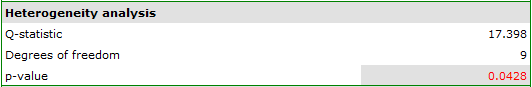
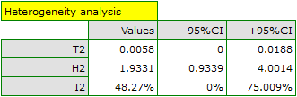
A statistically significant result of Q statistic was obtained (p=0.0428). The variance of the observed effects is non-zero (T2=0.0058), and the coefficient I2=48.27%, indicates moderate heterogeneity between studies. Only the confidence interval for the H2 coefficient finds insignificant variability between studies (the range for this coefficient is [0.93-4.00]). With these results in mind, it is important to consider whether the collected papers can be summarized by one overall result (shared relative risk) or whether it is worthwhile to determine a more homogeneous group of papers and perform the analysis again.

PQStat - Baza Wiedzy

Narzędzia użytkownika

Narzędzia witryny

Pasek boczny

Heterogeneity testing

Narzędzia strony