PQStat - Baza Wiedzy

The Intraclass Correlation Coefficient and a test to examine its significance

The intraclass correlation coefficient is used when the measurement of variables is done by a few „raters” ( $k\geq2$ ). It measures the strength of interrater reliability $-$ the degree of its assessment concordance.

Since it can be determined in several different situations, there are several variations depending on the model and the type of concordance. Depending on the variability present in the data, we can distinguish between 2 main research models and 2 types of concordance.

Model 1

For each of the $n$ randomly selected judged objects, a set of $k$ judges is randomly selected from the population of judges. Whereby for each object a different set of $k$ judges can be drawn.

The ICC coefficient is then determined by the random model ANOVA for independent groups. The question of the reliability of a single judge's ratings is answered by ICC(1,1) given by the formula:

$\begin{displaymath} ICC(1,1)=\frac{MS_{WG}-MS_{BG}}{MS_{WG}+(k-1)MS_{BG}}. \end{displaymath}$

To estimate the reliability of scores that are the average of the judges' ratings (for $k$ judges), determine ICC(1,k) given by the formula:

$\begin{displaymath}ICC(1,k)=\frac{MS_{WG}-MS_{BG}}{MS_{WG}},\end{displaymath}$

where:

$MS_{WG}$ – mean of squares within groups,

$MS_{BG}$ – mean of squares between objects.

Model 2

A set of $k$ judges is randomly selected from a population of judges and each judge evaluates all $n$ random objects. The ICC coefficient is then determined in a random model ANOVA for dependent groups.

Depending on the type of concordance we are looking for, we can estimate: absolute agreement, i.e., if the judges agree absolutely, they give exactly the same ratings, e.g., perfectly concordant will be such ratings given by a pair of judges (2,2), (5,5), (8,8); or consistency, i.e., the judges may use different ranges of values but beyond this shift there should be no differences to keep the verdict consistent, e.g., perfectly consistent will be such ratings given by a pair of judges (2,5), (5,8), (8,11).

Absolute agreement

The question about the reliability of a single judge's ratings is answered by ICC(2,1) given by the formula:

$\begin{displaymath} ICC(2,1)=\frac{MS_{BS}-MS_{res}}{MS_{BS}+(k-1)MS_{res}+\frac{k}{n}(MS_{BC}-MS_{res})}. \end{displaymath}$

To estimate the reliability of scores that are the average of the judges' ratings (for $k$ judges), determine ICC(2,k) given by the formula:

$\begin{displaymath}ICC(2,k)=\frac{MS_{BS}-MS_{res}}{MS_{BS}+(MS_{BC}-MS_{res})/n},\end{displaymath}$

where:

$MS_{BC}$ – the mean of squares between judges,

$MS_{BS}$ – the mean of squares between objects,

$MS_{res}$ – mean of squares for the residuals.

Consistency

The question about the reliability of a single judge's ratings is answered by ICC(2,1) given by the formula:

$\begin{displaymath} ICC(2,1)=\frac{MS_{BS}-MS_{res}}{MS_{BS}+(k-1)MS_{res}}, \end{displaymath}$

To estimate the reliability of scores that are the average of the judges' ratings (for $k$ judges), determine ICC(2,k) given by the formula:

$\begin{displaymath}ICC(2,k)=\frac{MS_{BS}-MS_{res}}{MS_{BS}},\end{displaymath}$

where:

$MS_{BS}$ – the mean of squares between objects,

$MS_{res}$ – mean of squares for the residuals.

Note

Sometimes, there is a need to consider model 3 ¹⁾, i.e., a set of $k$ judges is selected and each judge evaluates all $n$ random objects. The concordance score applies only to these particular $k$ judges. The ICC coefficient is then determined in a mixed model (since the randomness only affects the objects and not the judges). Since we are ignoring the variability concerning the judges, we are examining consistency (rather than absolute agreement) and the coefficients from the second model may apply: ICC(2,1) and ICC (2,k), since they are the same as the coefficients ICC(3,1) and ICC (3,k) desired in this case under the assumption of no interaction between objects and judges.

Note

We interpret the value $ICC\in<-1; 1>$ as follows:

$ICC\approx1$ it is an strong concordance of objects assessment made by judgess; it is especially reflected in a high-variance between objects (a significant means difference between $n$ objects) and a low-variance between judges assessments (a small means difference of assessments designated by $k$ judges);
$ICC\approx-1$ a negative intraclass coefficient is treated in the same ways as $r_{ICC}\approx0$ ;
$ICC\approx0$ denotes a lack of concordance in the judges' evaluations of individual objects, as reflected by low variance between objects (a small difference in means between $n$ objects) and high variance between judges' evaluations (a significant difference in mean scores determined for $k$ judges).

F-test for testing the significance of intraclass correlation coefficient

Basic assumptions:

measurement on an interval scale,
the normal distribution for all variables which are the differences of measurement pairs (or the normal distribution for an analysed variable in each measurement),
for model 1 - independent model, for model 2 / 3 - dependent model.

Hypotheses:

$\begin{array}{cl} \mathcal{H}_0: & ICC=0\\ \mathcal{H}_1: & ICC\neq 0 \quad(ICC=1) \end{array}$

The test statistic has the form:

$\begin{displaymath} F=\frac{MS_{BS}}{MS_{res}} - \textrm{in the dependent model,} \end{displaymath}$

or

$\begin{displaymath} F=\frac{MS_{WG}}{MS_{BG}} - \textrm{in the independent model.} \end{displaymath}$

This statistic has the F Snedecor distribution with the number of degrees of freedom defined in the model.

The p-value, designated on the basis of the test statistic, is compared with the significance level $\alpha$ :

$\begin{array}{ccl} $ if $ p \le \alpha & \Longrightarrow & $ reject $ \mathcal{H}_0 $ and accept $ \mathcal{H}_1, \\ $ if $ p > \alpha & \Longrightarrow & $ there is no reason to reject $ \mathcal{H}_0. \\ \end{array}$

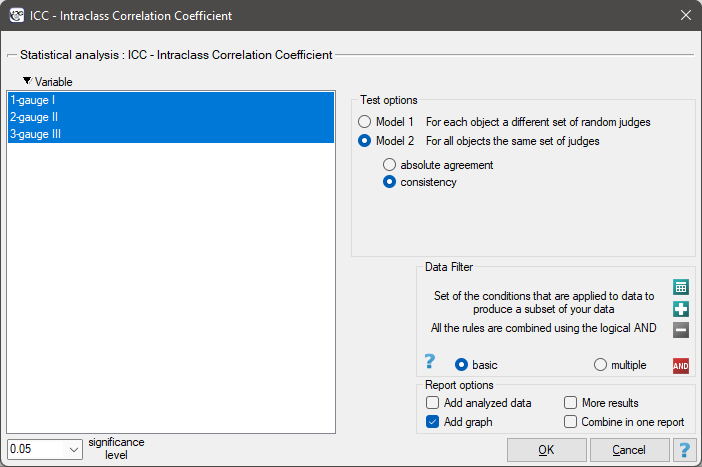
The settings window with the ICC – Intraclass Correlation Coefficient can be opened in Statistics menu→Parametric tests→ICC – Intraclass Correlation Coefficient or in ''Wizard''.

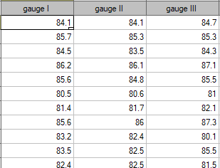
EXAMPLE (sound intensity.pqs file)

In order to effectively care for the hearing of workers in the workplace, it is first necessary to reliably estimate the sound intensity in the various areas where people are present. One company decided to conduct an experiment before choosing a sound intensity meter (sonograph). Measurements of sound intensity were made at 42 randomly selected measurement points in the plant using 3 drawn analog sonographs and 3 randomly selected digital sonographs. A part of collected measurements is presented in the table below.

To find out which type of instrument (analog or digital) will better accomplish the task at hand, the ICC in model 2 should be determined by examining the absolute agreement. The type of meter with the higher ICC will have more reliable measurements and will therefore be used in the future.

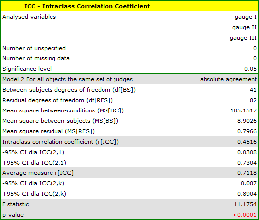
The analysis performed for the analog meters shows significant consistency of the measurements (p<0.0001). The reliability of the measurement made by the analog meter is ICC(2,1) = 0.45, while the reliability of the measurement that is the average of the measurements made by the 3 analog meters is slightly higher and is ICC(2,k) = 0.71. However, the lower limit of the 95 percent confidence interval for these coefficients is disturbingly low.

A similar analysis performed for digital meters produced better results. The model is again statistically significant, but the ICC coefficients and their confidence intervals are much higher than for analog meters, so the absolute agreement obtained is higher ICC(2,1) = 0.73, ICC(2,k) = 0.89.

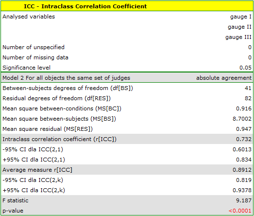
Therefore, eventually digital meters will be used in the workplace.

The agreement of the results obtained for the digital meters is shown in a dot plot, where each measurement point is described by the sound intensity value obtained for each meter.

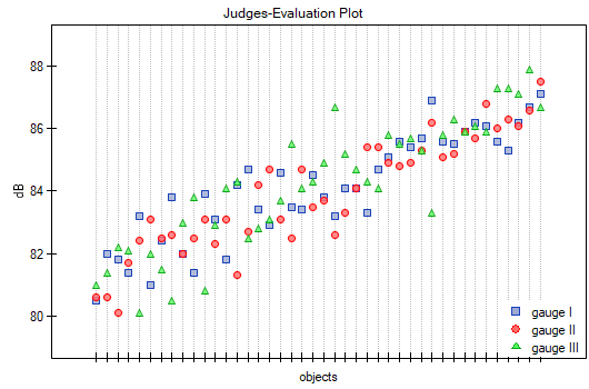
By presenting a graph for the previously sorted data according to the average value of the sound intensity, one can check whether the degree of agreement increases or decreases as the sound intensity increases. In the case of our data, a slightly higher correspondence (closeness of positions of points on the graph) is observed at high sound intensities.

Similarly, the consistency of the results obtained can be observed in the Blanda-Altmana graphs²⁾ constructed separately for each pair of meters. The graph for Meter I and Meter II is shown below.

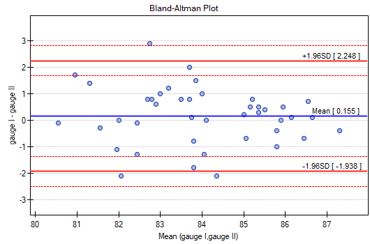
Here, too, we observe higher agreement (points are concentrated near the horizontal axis y=0) for higher sound intensity values.

Note

If the researcher was not concerned with estimating the actual sound level at the worksite, but wanted to identify where the sound level was higher than at other sites or to see if the sound level varied over time, then Model 2, which tests consistency, would be a sufficient model.

¹⁾

Shrout P.E., and Fleiss J.L (1979), Intraclass correlations: uses in assessing rater reliability. Psychological Bulletin, 86, 420-428

²⁾

Bland J.M., Altman D.G. (1999), Measuring agreement in method comparison studies. Statistical Methods in Medical Research 8:135-160.

PQStat - Baza Wiedzy

Narzędzia użytkownika

Narzędzia witryny

Pasek boczny

The Intraclass Correlation Coefficient and a test to examine its significance

Narzędzia strony