PQStat - Baza Wiedzy

Comparison of logistic regression models

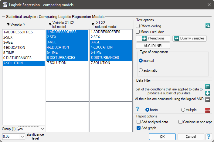
The window with settings for model comparison is accessed via the menu Advanced Statistics→Multivariate models→Logistic regression – comparing models

Due to the possibility of simultaneous analysis of many independent variables in one logistic regression model, similarly to the case of multiple linear regression, there is a problem of selection of an optimum model. When choosing independent variables one has to remember to put into the model variables strongly correlated with the dependent variable and weakly correlated with one another.

When comparing models with different numbers of independent variables, we pay attention to model fit and information criteria. For each model we also calculate the maximum of the credibility function, which we then compare using the credibility quotient test.

Hypotheses:

$\begin{array}{cc} \mathcal{H}_0: & L_{FM}=L_{RM},\\ \mathcal{H}_1: & L_{FM}\ne L_{RM}, \end{array}$

where:

$L_{FM}, L_{RM}$ – the maximum of likelihood function in compared models (full and reduced).

The test statistic has the form presented below:

$\begin{displaymath} \chi^2=-2\ln(L_{RM}/L_{FM})=-2\ln(L_{RM})-(-2\ln(L_{FM})) \end{displaymath}$

The statistic asymptotically (for large sizes) has the Chi-square distribution with $df=k_{FM}-k_{RM}$ degrees of freedom, where $k_{FM}$ i $k_{RM}$ is the number of estimated parameters in compared models.

The p-value, designated on the basis of the test statistic, is compared with the significance level $\alpha$ :

$\begin{array}{ccl} $ if $ p \le \alpha & \Longrightarrow & $ reject $ \mathcal{H}_0 $ and accept $ \mathcal{H}_1, \\ $ if $ p > \alpha & \Longrightarrow & $ there is no reason to reject $ \mathcal{H}_0. \\ \end{array}$

We make the decision about which model to choose on the basis of the size $R_{Pseudo}^2$ , $R^2_{Nagelkerke}$ , $R^2_{Cox-Snell}$ and the result of the Likelihood Ratio test which compares the subsequently created (neighboring) models. If the compared models do not differ significantly, we should select the one with a smaller number of variables. This is because a lack of a difference means that the variables present in the full model but absent in the reduced model do not carry significant information. However, if the difference is statistically significant, it means that one of them (the one with the greater number of variables, with a greater $R^2$ and a lower information criterion value of AIC, AICc or BIC) is significantly better than the other one.

Comparison the predictive value of models.

The regression models that are built allow to predict the probability of occurrence of the studied event based on the analyzed independent variables. When many variables (factors) that increase the risk of an event are already known, then an important criterion for a new candidate risk factor is the improvement in prediction performance when that factor is added to the model. To establish the point, let's use an example. Suppose we are studying risk factors for coronary heart disease. Known risk factors for this disease include age, systolic and diastolic blood pressure values, obesity, cholesterol, or smoking. However, the researchers are interested in how much the inclusion of individual factors in the regression model will significantly improve disease risk estimates. Risk factors added to a model will have predictive value if the new and larger model (which includes these factors) shows better predictive value than a model without them. The predictive value of the model is derived from the determined value of the predicted probability of an event, in this case coronary artery disease. This value is determined from the model for each individual tested. The closer the predicted probability is to 1, the more likely the disease is. Based on the predicted probability, the value of the AUC area under the ROC curve can be determined and compared between different models, as well as the $NRI$ and $IDI$ coefficient.

Change of the area under the ROC curve

The ROC curve in logistic regression models is constructed based on the classification of cases into a group experiencing an event or not, and the predicted probability of the dependent variable $P$ . The larger the area under the curve, the more accurately the probability determined by the model predicts the actual occurrence of the event. If we are comparing models built on the basis of a larger or smaller number of predictors, then by comparing the size of the area under the curve we can check whether the addition of factors has significantly improved the prediction of the model.

Hypotheses:

$\begin{array}{cl} \mathcal{H}_0: & AUC_{FM}=AUC_{RM}, \mathcal{H}_1: & AUC_{FM}\neq AUC_{RM}. \end{array}$

For a method of determining the test statistic based on DeLong's method, check out Comparing ROC curves.

The p-value, designated on the basis of the test statistic, is compared with the significance level $\alpha$ :

$\begin{array}{ccl} $ if $ p \le \alpha & \Longrightarrow & $ reject $ \mathcal{H}_0 $ and accept $ \mathcal{H}_1, \\ $ if $ p > \alpha & \Longrightarrow & $ there is no reason to reject $ \mathcal{H}_0. \\ \end{array}$

Net reclassification improvement

This measure is denoted by the acronym $NRI$ The $NRI$ focuses on the reclassification table describing the upward or downward shift in probability values when a new factor is added to the model. It is determined based on two separate factors, i.e., a factor determined separately for subjects experiencing the event (1) and separately for those not experiencing the event (0). The $NRI$ can be determined with a given division of the predicted probability into categories (categorical $NRI$ ) or without the need to determine the categories (continuous $NRI$ ).

NRI categorical requires an arbitrary determination of the division of probability values predicted from the model. There can be a maximum of 9 split points given, and thus a maximum of 10 predicted categories. However, one or two split points are most commonly used. At the same time, it should be noted that the values of the categorical $NRI$ can be compared with each other only if they were based on the same split points. To illustrate the situation, let's establish two example probability split points: 0.1 and 0.3. If a test person in the „old” (smaller) model received a probability below 0.1, and in the „new model” (increased by a new potential risk factor) probability located between 0.1 and 0.3, it means that the person was reclassified upwards (table, situation 1). If the probability values from both models are in the same range, then the person is not reclassified (table, situation 2), whereas if the probability from the „new” model is lower than that from the „old” model, then the person is reclassified downwards (table, situation 3).

$\begin{tabular}{|c|c|c||c|c||c|c|} \hline regression models&\multicolumn{2}{|c||}{situation 1}&\multicolumn{2}{|c||}{situation 2}&\multicolumn{2}{|c|}{situation 3}\\\hline predicted probability&"old"&"new"&"old"&"new"&"old"&"new"\\\hline [0.3 do 1]&&&&&$\oplus$&\\\hline [0.1; 0.3)&&$\oplus$&$\oplus$&$\oplus$&&$\oplus$\\\hline [0; 0.1)&$\oplus$&&&&&\\\hline \end{tabular}$

NRI continuous does not require an arbitrary designation of categories, since any, even the smallest, change in probability up or down from the probability designated in the „old model” is treated as a transition to the next category. Thus, there are infinitely many categories, just as there are many possible changes.

Note

Use of continuous $NRI$ does not require arbitrary definition of probability split points, but even small changes in risk (not reflected in clinical observations) can increase or decrease this ratio. The categorical $NRI$ factor allows only changes that are important to the investigator to reflect changes that involve exceeding preset event risk values (predicted probability values).

To determine $NRI$ we define:

$\hat{p}_{up,events}=\frac{\#events_{up}}{\#events}$

$\hat{p}_{down,events}=\frac{\#events_{down}}{\#events}$

$\hat{p}_{up,nonevents}=\frac{\#nonevents_{up}}{\#nonevents}$

$\hat{p}_{down,nonevents}=\frac{\#nonevents_{down}}{\#nonevents}$

where:

$\#events_{up}$ – the number of subjects in the group experiencing the event for whom there was an upward change of at least one category in the predicted probability,

$\#events_{down}$ – the number of subjects in the group experiencing the event for whom there was at least one downward change in predicted probability,

$\#events$ – number of objects in the group experiencing the event,

$\#nonevents_{up}$ – The number of subjects in the group not experiencing the event for whom there was an upward change of at least one category in the predicted probability,

$\#nonevents_{down}$ – The number of subjects in the group not experiencing the event for whom there was at least one downward change in predicted probability,

$\#nonevents$ – number of objects in the group not experiencing the event.

The overall $NRI$ and coefficients expressing the percentage change in classification are determined from the formula:

$\begin{displaymath} NRI=\left(\hat{p}_{up,events}-\hat{p}_{down,events}\right)-\left(\hat{p}_{up,nonevents}-\hat{p}_{down,nonevents}\right) \end{displaymath}$

$\begin{displaymath} NRI_{events}=\hat{p}_{up,events}-\hat{p}_{down,events}, \quad NRI_{nonevents}=\hat{p}_{down,nonevents}-\hat{p}_{up,nonevents}, \end{displaymath}$

The $NRI_{events}$ coefficient can be interpreted as the net percentage of correctly reclassified individuals with an event, and $NRI_{nonevents}$ as the net percentage of correctly reclassified individuals without an event. The overall coefficient $NRI$ is expressed as the sum of the coefficients $NRI_{events}$ and $NRI_{nonevents}$ making it a coefficient implicitly weighted by event frequency and cannot be interpreted as a percentage.

The $NRI_{events}$ coefficientsbelong to the range from-1 to 1 (from -100% to 100%), and the overall coefficients of $NRI$ belong to the range from -2 to 2. Positive values of the coefficients indicate favorable reclassification, and negative values indicate unfavorable reclassification due to the addition of a new variable to the model.

Z test for significance of NRI coefficient

Using this test, we examine whether the change in classification expressed by the $NRI$ coefficient was significant.

Hypotheses:

$\begin{array}{cl} \mathcal{H}_0: & NRI=0,\\ \mathcal{H}_1: & NRI\neq 0. \end{array}$

The test statistic has the form:

$\begin{displaymath} Z=\frac{NRI}{SE(NRI)} \end{displaymath}$

where:

$\begin{array}{cl} SE(NRI)= & [\left(\frac{\#events_{up} + \#events_{down}}{\#events^2}-\frac{(\#events_{up} + \#events_{down})^2}{\#events^3}\right)+\\ & +\left(\frac{\#nonevents_{down} + \#nonevents_{up}}{\#nonevents^2}-\frac{(\#nonevents_{down} + \#nonevents_{up})^2}{\#nonevents^3}\right)]^{1/2} \end{array}$

The $Z$ statistic asymptotically (for large sample sizes) has the normal distribution.

The p-value, designated on the basis of the test statistic, is compared with the significance level $\alpha$ :

$\begin{array}{ccl} $ if $ p \le \alpha & \Longrightarrow & $ reject $ \mathcal{H}_0 $ and accept $ \mathcal{H}_1, \\ $ if $ p > \alpha & \Longrightarrow & $ there is no reason to reject $ \mathcal{H}_0. \\ \end{array}$

Integrated Discrimination Improvement

This measure is denoted by the abbreviation $IDI$ . The $IDI$ coefficients indicate the difference between the value of the average change in the predicted probability between the group of objects experiencing the event and the group of objects that did not experience the event.

$\begin{displaymath} IDI=\overline{p(diff)}_{events}-\overline{p(diff)}_{nonevents} \end{displaymath}$

where:

$\overline{p(diff)}_{events}$ – The mean of the difference in predicted probability values between the regression models („old” and „new”) for objects that experienced the event,

$\overline{p(diff)}_{nonevents}$ – The mean of the difference in predicted probability values between the regression models („old” and „new”) for objects that did not experience the event.

Z test for significance of IDI coefficient

Using this test, we examine whether the difference between the value of the mean change in predicted probability between the group of subjects experiencing the event and the subjects not experiencing the event, as expressed by the $IDI$ coefficient, was significant.

Hypotheses:

$\begin{array}{cl} \mathcal{H}_0: & IDI=0,\\ \mathcal{H}_1: & IDI\neq 0. \end{array}$

The test statistic is of the form:

$\begin{displaymath} Z=\frac{IDI}{SE(IDI)} \end{displaymath}$

where:

$SE(IDI)=\sqrt{\frac{sd(diff)^2_{events}}{\#events}+\frac{sd(diff)^2_{nonevents}}{\#nonevents}}$

The $Z$ statistic asymptotically (for large sample sizes) has the normal distribution.

The p-value, designated on the basis of the test statistic, is compared with the significance level $\alpha$ :

$\begin{array}{ccl} $ if $ p \le \alpha & \Longrightarrow & $ reject $ \mathcal{H}_0 $ and accept $ \mathcal{H}_1, \\ $ if $ p > \alpha & \Longrightarrow & $ there is no reason to reject $ \mathcal{H}_0. \\ \end{array}$

In the program PQStat the comparison of models can be done manually or automatically.

Manual model comparison – construction of 2 models:
- a full model – a model with a greater number of variables,
- a reduced model – a model with a smaller number of variables – such a model is created from the full model by removing those variables which are superfluous from the perspective of studying a given phenomenon.

The choice of independent variables in the compared models and, subsequently, the choice of a better model on the basis of the results of the comparison, is made by the researcher.

Automatic model comparison is done in several steps:

[step 1] Constructing the model with the use of all variables.
[step 2] Removing one variable from the model. The removed variable is the one which, from the statistical point of view, contributes the least information to the current model.
[step 3] A comparison of the full and the reduced model.
[step 4] Removing another variable from the model. The removed variable is the one which, from the statistical point of view, contributes the least information to the current model.
[step 5] A comparison of the previous and the newly reduced model.
[…]

In that way numerous, ever smaller models are created. The last model only contains 1 independent variable.

EXAMPLE cont. (task.pqs file)

In the experiment made with the purpose to study, for 130 people of the teaching set, the concentration abilities a logistic regression model was constructed on the basis of the following variables:

dependent variable: SOLUTION (yes/no) - information about whether the task was correctly solved or not;

independent variables:

ADDRESSOFRES (1=city/0=village),

SEX (1=female/0=male),

AGE (in years),

EDUCATION (1=primary, 2=vocational, 3=secondary, 4=tertiary),

TIME needed for the completion of the task (in minutes),

DISTURBANCES (1=yes/0=no).

Let us check if all independent variables are indispensible in the model.

Manual model comparison.

On the basis of the previously constructed full model we can suspect that the variables: ADDRESSOFRES and SEX have little influence on the constructed model (i.e. we cannot successfully make classifications on the basis of those variables). Let us check if, from the statistical point of view, the full model is better than the model from which the two variables have been removed.

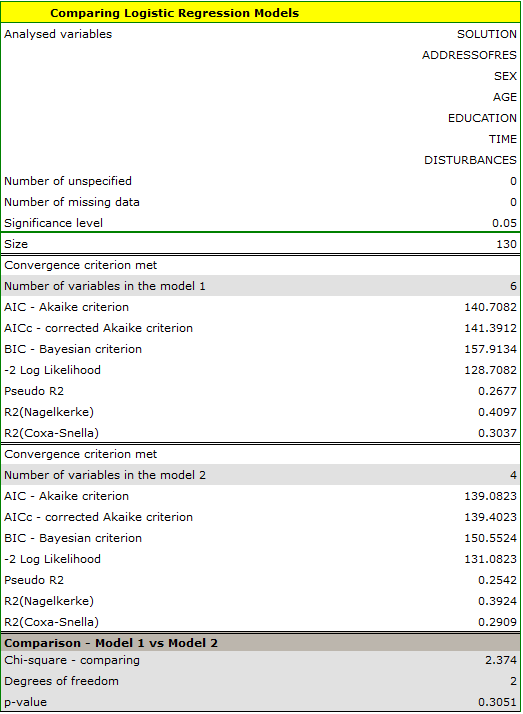
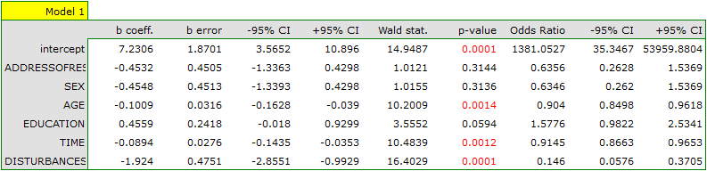
The results of the Likelihood Ratio test ( $p=0.3051$ ) indicates that there is no basis for believing that a full model is better than a reduced one. Therefore, with a slight worsening of model adequacy, the address of residence and the sex can be omitted.

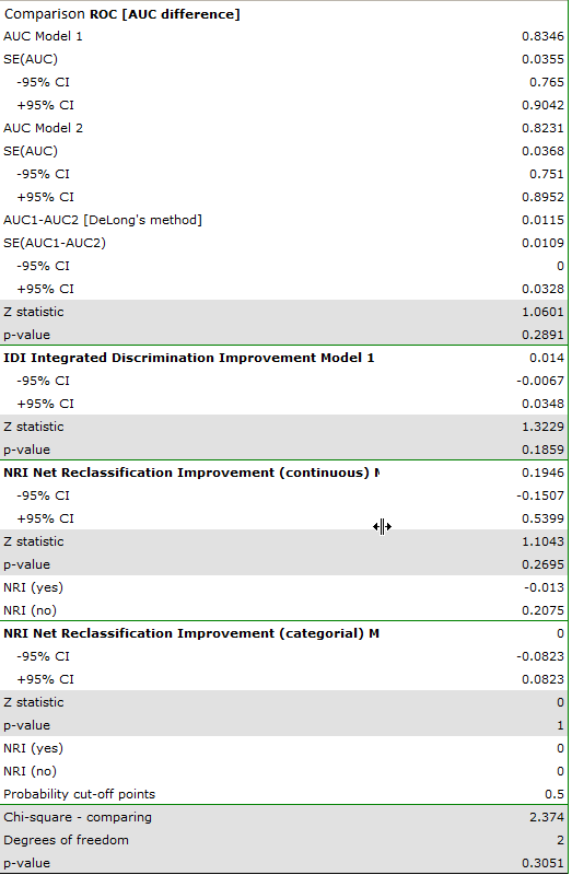
We can compare the two models in terms of classification ability by comparing the ROC curves for these models, NRI and IDI value. To do so, we select the appropriate option in the analysis window. The resulting report, like the previous one, indicates that the models do not differ in prediction quality i.e. the p-values for the comparison of ROC curves and for the evaluation of NRI and IDI indices are statistically insignificant. We therefore decide to omit gender and place of residence from the final model.

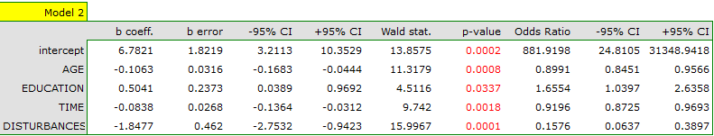
Automatic model comparison.

For automatic model comparison, we obtained very similar results. The best model is the model built on the independent variables: AGE, EDUCATION, TIME OF SOLUTION, and DISTURBANCES. Based on the above analyses, from a statistical point of view, the optimal model is one containing the 4 most important independent variables: AGE, EDUCATION, RESOLUTION TIME, and DISTURBANCES. Its detailed analysis can be done in the Logistic Regression module. However, the final decision which model to choose is up to the experimenter.

EXAMPLE (Heart.pqs file)

Risk factors for certain heart disease such as age, bmi, smoking, LDL fraction cholesterol, HDL fraction cholesterol, and hypertension were examined. From the researcher's point of view, it was interesting to determine how much information about smoking could improve the prediction of the occurrence of the disease under study.

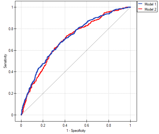
We compare a logistic regression model describing the risk of heart disease based on all study variables with a model without smoking information. In the analysis window, we select the options related to the prediction evaluation, namely the ROC curve and the NRI coefficients. In addition, we indicate to include all proposed graphs in the report.

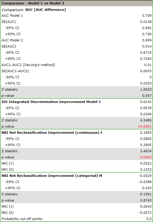
Analysis of the report indicates important differences in prediction as a result of adding smoking information to the model, although they are not significant in describing the ROC curve (p=0.057).

The continuous IDI and NRI coefficient values indicate a statistically significant and favorable change (the values of these coefficients are positive with p<0.05). The prognosis for those with heart disease improved by more than 5% and those without heart disease by more than 13% (NRI(sick)=0.0522, NRI(healthy)=0.1333)) as a result of including information about smoking.

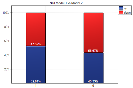
We also see the conclusions drawn from the NRI in the graph. We see an increase in the model-predicted probability of disease in diseased individuals (more individuals were reclassified upward than downward 52.61% vs 47.39%) while a decrease in the probability applies more to healthy individuals (more individuals were reclassified downward than upward 56.67% vs 43.33%). It is also possible to determine a categorical NRI, but to do so, one would first need to determine the model-determined probability cut-off points accepted in the heart disease literature.

PQStat - Baza Wiedzy

Narzędzia użytkownika

Narzędzia witryny

Pasek boczny

Comparison of logistic regression models

Narzędzia strony