PQStat - Baza Wiedzy

EXAMPLE (anomaly.pqs file)

Studies have been conducted for the purpose of identifying the risk factors for a certain rare congenital anomaly in children. 395 mothers of children with that anomaly and 375 of healthy children have participated in that study. The gathered data are: address of residence, child's sex, child's weight at birth, mother's age, number of pregnancy, previous spontaneous abortions, respiratory tract infections, smoking, mother's education.

We construct a logistic regression model to check which variables may have a significant influence on the occurrence of the anomaly. The dependent variable is the column GROUP, the distinguished values in that variable as are the cases, that are mothers of children with anomaly. The following variables are independent variables:

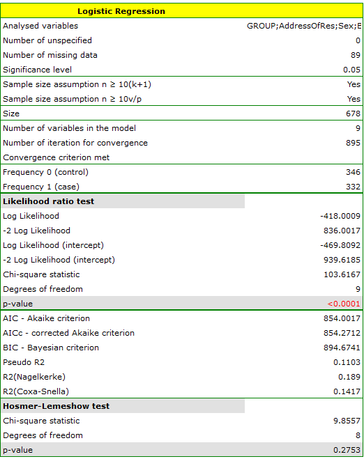
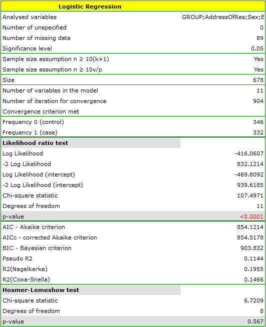
The quality of model goodness of fit is not high (, i ). At the same time the model is statistically significant (value of the Likelihood Ratio test), which means that a part of the independent variables in the model is statistically significant. The result of the Hosmer-Lemeshow test points to a lack of significance (). However, in the case of the Hosmer-Lemeshow test we ought to remember that a lack of significance is desired as it indicates a similarity of the observed sizes and of predicted probability.

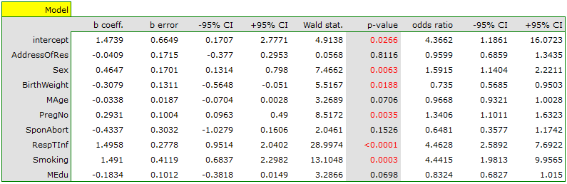
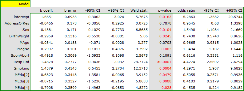
An interpretation of particular variables in the model starts from checking their significance. In this case the variables which are significantly related to the occurrence of the anomaly are:

The studied congenital anomaly is a rare anomaly but the odds of its occurrence depend on the variables listed above in the manner described by the odds ratio:

• variable Sex: \textendash the odds of the occurrence of the anomaly in a boy is times greater than in a girl;
• variable BirthWeight: \textendash the higher the birth weight the smaller the odds of the occurrence of the anomaly in a child;
• variable PregNo: \textendash the odds of the occurrence of the anomaly in a child is times greater with each subsequent pregnancy;
• variable RespTInf: \textendash the odds of the occurrence of the anomaly in a child if the mother had a respiratory tract infection during the pregnancy is times greater than in a mother who did not have such an infection during the pregnancy;
• variable Smoking: \textendash a mother who smokes when pregnant increases the risk of the occurrence of the anomaly in her child times.

In the case of statistically insignificant variables the confidence interval for the Odds Ratio contains 1 which means that the variables neither increase nor decrease the odds of the occurrence of the studied anomaly. Therefore, we cannot interpret the obtained ratio in a manner similar to the case of statistically significant variables.

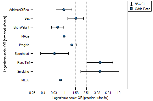
The influence of particular independent variables on the occurrence of the anomaly can also be described with the help of a chart concerning the odds ratio:

EXAMPLE continued (anomaly.pqs file)

Let us once more construct a logistic regression model, however, this time let us divide the variable mother's education into dummy variables (with dummy coding). With this operation we lose the information about the ordering of the category of education but we gain the possibility of a more in-depth analysis of particular categories. The breakdown into dummy variables is done by selecting Dummy var. in the analysis window.:

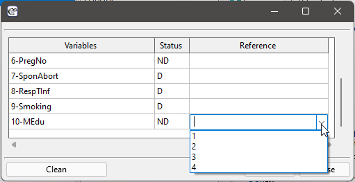
The primary education variable is missing as it will constitute the reference category.

As a result the variables which describe education become statistically significant. The goodness of fit of the model does not change much but the manner of interpretation of the the odds ratio for education does change:

The odds of the occurrence of the studied anomaly in each education category is always compared with the odds of the occurrence of the anomaly in the case of primary education. We can see that for more educated the mother, the odds is lower. For a mother with:

• vocational education the odds of the occurrence of the anomaly in a child is 0.51 of the odds for a mother with primary education;
• secondary education the odds of the occurrence of the anomaly in a child is 0.42 of the odds for a mother with primary education;
• tertiary education the odds of the occurrence of the anomaly in a child is 0.45 of the odds for a mother with primary education;

EXAMPLE (task.pqs file)

An experiment has been made with the purpose of studying the ability to concentrate of a group of adults in an uncomfortable situation. 190 people have taken part in the experiment (130 people are the teaching set, 40 people are the test set). Each person was assigned a certain task the completion of which requried concentration. During the experiment some people were subject to a disturbing agent in the form of temperature increase to 32 degrees Celsius. The participants were also asked about their address of residence, sex, age, and education. The time for the completion of the task was limited to 45 minutes. In the case of participants who completed the task before the deadline, the actual time devoted to the completion of the task was recorded. We will perform all our calculations only for those belonging to the teaching set. }

Variable SOLUTION (yes/no) contains the result of the experiment, i.e. the information about whether the task was solved correctly or not. The remaining variables which could have influenced the result of the experiment are:

On the basis of all those variables a logistic regression model was built in which the distinguished state of the variable SOLUTION was set to „yes”.

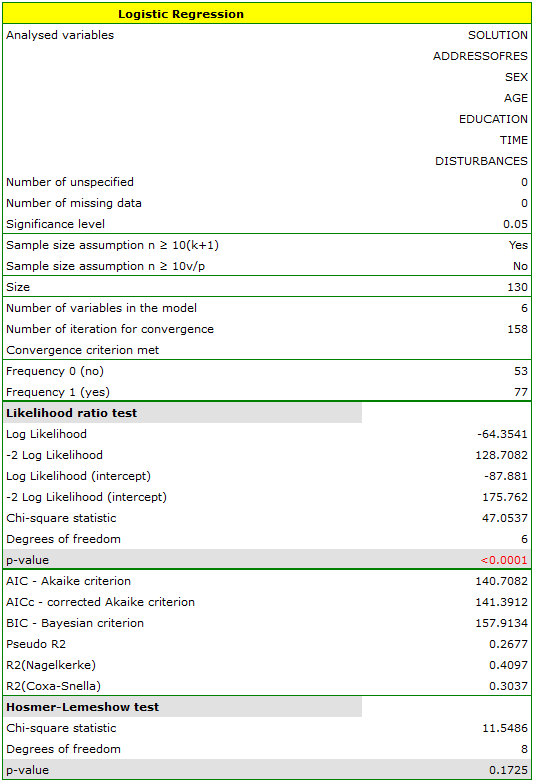
The adequacy quality is described by the coefficients: , i . The sufficient adequacy is also indicated by the result of the Hosmer-Lemeshow test . The whole model is statistically significant, which is indicated by the result of the Likelihood Ratio test .

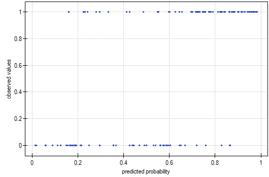
The observed values and predicted probability can be observed on the chart:

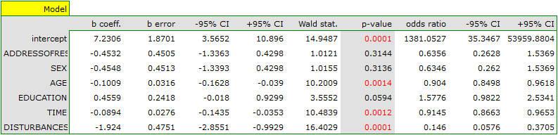
In the model the variables which have a significant influence on the result are:

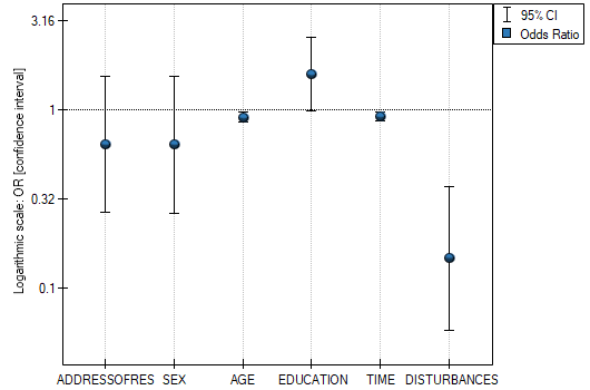
What is more, the younger the person who solves the task the shorter the time needed for the completion of the task, and if there is no disturbing agent, the probability of correct solution is greater:

The obtained results of the Odds Ratio are presented on the chart below:

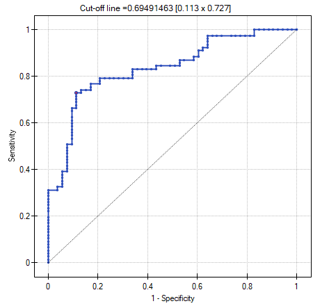
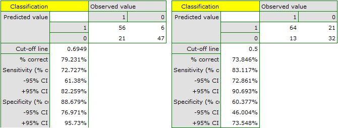
Should the model be used for prediction, one should pay attention to the quality of classification. For that purpose we calculate the ROC curves.

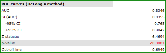
The result seems satisfactory. The area under the curve is and is statistically greater than , so classification is possible on the basis of the constructed model. The suggested cut-off point for the ROC curve is and is slightly higher than the standard level used in regression, i.e. . The classification determined from this cut-off point yields of cases classified correctly, of which correctly classified yes values are (sensitivity), no values are (specificity). The classification derived from the standard value yields no less, of cases classified correctly, but it will yield more correctly classified yes values are , although less correctly classified no values are .

We can finish the analysis of classification at this stage or, if the result is not satisfactory, we can make a more detailed analysis of the ROC curve in module ROC curve.

As we have assumed that classification on the basis of that model is satisfactory we can calculate the predicted value of a dependent variable for any conditions. Let us check what odds of solving the task has a person whose:

For that purpose, on the basis of the value of coefficient , we calculate the predicted probability (probability of receiving the answer „yes” on condition of defining the values of dependent variables):

As a result of the calculation the program will return the result:

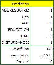
The obtained probability of solving the task is equal to , so, on the basis of the cut-off , the predicted result is \textendash which means the task was not solved correctly.