PQStat - Baza Wiedzy

The ANOVA for independent groups with F* and F" corrections

$F^*$ (Brown-Forsythe, 1974¹⁾) and $F''$ (Welch, 1951²⁾) Corrections concern ANOVA for independent groups and are calculated when the assumption of equality of variances is not met.

The test statistic is in the form of:

$\begin{displaymath} F^*=\frac{SS_{BG}}{\sum_{j=1}^k\left(1-\frac{n_j}{n}sd_j^2\right)}, \end{displaymath}$

$\begin{displaymath} F''=\frac{\frac{\sum_{j=1}^kw_j(\overline{x}_j-\widetilde{x})}{k-1}}{1+\frac{2(k-2)}{k^2-1}\sum_{j=1}^kh_j}, \end{displaymath}$

where:

$sd_j$ – group standard deviation $j$ ,

$w_j=\frac{n_j}{sd_j^2}$ – group weight $j$ ,

$\widetilde{x}$ – weighted mean,

$h_j=\frac{\left(1-\frac{w_j}{\sum_{j=1}^kw_j}\right)^2}{n_j-1}$ .

This statistic is subject toSnedecor's F distribution with $k-1$ and adjusted $df_{WG_k}$ degrees of freedom.

The p-value, designated on the basis of the test statistic, is compared with the significance level $\alpha$ :

$\begin{array}{ccl} $ if $ p \le \alpha & \Longrightarrow & $ reject $ \mathcal{H}_0 $ and accept $ \mathcal{H}_1, \\ $ if $ p > \alpha & \Longrightarrow & $ there is no reason to reject $ \mathcal{H}_0. \\ \end{array}$

POST-HOC Tests

Introduction to the contrasts and POST-HOC tests was done in chapter concerning one-way analysis of variance.

T2 Tamhane test

For simple and complex comparisons, equal-size groups as well as unequal-size groups, when the variances differ significantly (Tamhane A. C., 1977³⁾).

[i] The value of critical difference is calculated by using the following formula:

$\begin{displaymath} CD=\sqrt{F_{\alpha_{Sidak},1,df_v}}\cdot \sqrt{\left(\sum_{j=1}^k \frac{c_j^2sd_j^2}{n_j}\right)}, \end{displaymath}$

where:

$F_{\alpha_{Sidak},1,df_v}$ - is the critical value (statistics) of the Snedecor's F distribution for modified significance level $\alpha_{Sidak}$ and for degrees of freedom 1 and $df_{v}$ respectively,

$\alpha_{Sidak}=1-(1-\alpha)^{(1/k)}$ ,

$df_v=\frac{\left(\sum_{j=1}^k\frac{c_j^2sd_j^2}{n_j}\right)^2}{\sum_{j=1}^k\frac{c_j^4sd_j^4}{n_j^2(n_j-1)}}$

[ii] The test statistic is in the form of:

$\begin{displaymath} t=\frac{\left(\sum_{j=1}^k c_j\overline{x}_j\right)^2}{\sqrt{\left(\sum_{j=1}^k \frac{c_j^2sd_j^2}{n_j}\right)}}. \end{displaymath}$

This statistic is subject to the t-Student distribution with $df_v$ degrees of freedom, and p-value is adjusted by the number of possible simple comparisons.

BF test (Brown-Forsythe)

For simple and complex comparisons, equal-size groups as well as unequal-size groups, when the variances differ significantly (Brown M. B. i Forsythe A. B. (1974)⁴⁾).

[i] The value of critical difference is calculated by using the following formula:

$\begin{displaymath} CD=\sqrt{F_{\alpha,k-1,df_v}}\cdot \sqrt{(k-1)\left(\sum_{j=1}^k \frac{c_j^2sd_j^2}{n_j}\right)}, \end{displaymath}$

where:

$F_{\alpha,k-1,df_v}$ - is the critical value (statistics) of the Snedecor's F distribution for a given significance level $\alpha$ as well as $k-1$ and $df_v$ degrees of freedom.

[ii] The test statistic is in the form of:

$\begin{displaymath} F=\frac{\left(\sum_{j=1}^k c_j\overline{x}_j\right)^2}{(k-1)\left(\sum_{j=1}^k \frac{c_j^2sd_j^2}{n_j}\right)}. \end{displaymath}$ This statistic is subject to Snedecor's F distribution with $k-1$ and $df_v$ degrees of freedom.

GH test (Games-Howell).

For simple and complex comparisons, equal-size groups as well as unequal-size groups, when the variances differ significantly (Games P. A. i Howell J. F. 1976⁵⁾).

[i] The value of critical difference is calculated by using the following formula:

$\begin{displaymath} CD=\frac{q_{\alpha,k,df_v} \cdot \sqrt{\left(\sum_{j=1}^k \frac{c_j^2sd_j^2}{n_j}\right)}}{\sqrt{2}}, \end{displaymath}$

gdzie:

$q_{\alpha,k,df_v}$ - is the critical value (statistics) of the the distribution of the studentised interval for a given significance level $\alpha$ as well as $k$ and $df_v$ degrees of freedom.

[ii] The test statistic is in the form of:

$\begin{displaymath} q=\sqrt{2}\frac{\sum_{j=1}^k c_j\overline{x}_j}{\sqrt{\left(\sum_{j=1}^k \frac{c_j^2sd_j^2}{n_j}\right)}}. \end{displaymath}$ This statistic follows a studenty distribution with $k$ and $df_v$ degrees of freedom.

Trend test.

The test examining the presence of a trend can be calculated in the same situation as ANOVA for independent groups with correction $F^*$ and $F''$ , because it is based on the same assumptions, however, differently captures the alternative hypothesis - indicating the existence of a trend in the mean values for successive populations. The analysis of the trend of the arrangement of means is based on contrasts (T2 Tamhane). By creating appropriate contrasts you can study any type of trend e.g. linear, quadratic, cubic, etc. A table of sample contrast values for certain trends can be found in the description trend test for Ona-Way ANOVA.

Linear trend

A linear trend, like other trends, can be analyzed by entering the appropriate contrast values. However, if the direction of the linear trend is known, simply use the Linear Trend option and indicate the expected order of the populations by assigning them consecutive natural numbers.

The analysis is performed based on linear contrast, i.e., the groups indicated according to the natural ordering are assigned appropriate contrast values and the T2 Tamhane statistic is calculated.

With the expected direction of the trend being known, the alternative hypothesis is one-sided and the one-sided value of $p$ is subject to interpretation. The interpretation of the two-sided value of $p$ means that the researcher does not know (does not assume) the direction of the possible trend.

The p-value, designated on the basis of the test statistic, is compared with the significance level $\alpha$ :

$\begin{array}{ccl} $ if $ p \le \alpha & \Longrightarrow & $ reject $ \mathcal{H}_0 $ and accept $ \mathcal{H}_1, \\ $ if $ p > \alpha & \Longrightarrow & $ there is no reason to reject $ \mathcal{H}_0. \\ \end{array}$

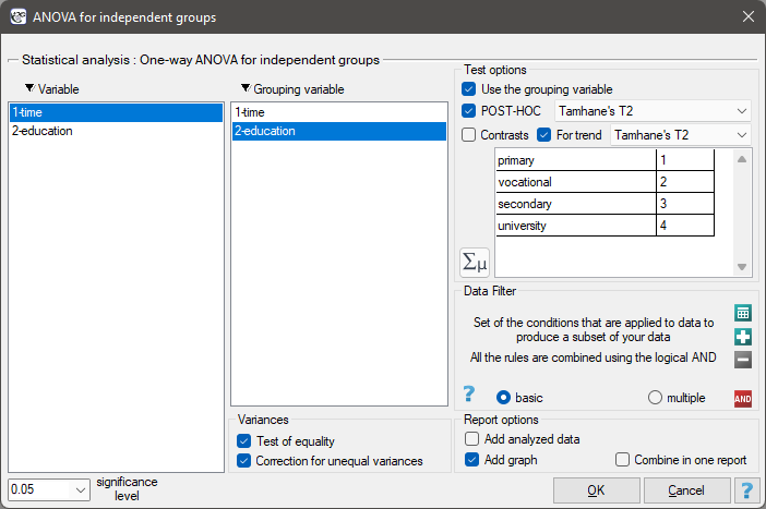
Settings window for the One-way ANOVA for independent groups with F* and F„ adjustments is opened via menu Statistics→Parametric tests→ANOVA for independent groups or via the ''Wizard''.

EXAMPLE (unemployment.pqs file)

There are many factors that control the time it takes to find a job during an economic crisis. One of the most important may be the level of education. Sample data on education and time (in months) of unemployment are gathered in the file. We want to see if there are differences in average job search time for different education categories.

Hypotheses:

$\begin{array}{cl} \mathcal{H}_0: & $average job search time is the same $\\ & $for every category of education,$\\ \mathcal{H}_1: & $at least one education category (one population)$\\ & $ have a different average job search time.$\\ \end{array}$

Due to differences in variance between populations (for Levene test $p=0.0001$ and for Brown-Forsythe test $p=0.0002$ ):

the analysis is performed with the correction of various variances enabled. The obtained result of the adjusted $F$ statistic is shown below.

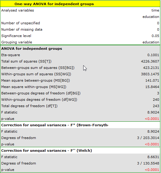
Comparing $p<0.0001$ (for the $F^*$ test) and $p<0.0001$ (for the $F''$ test) with a significance level of $\alpha=0.05$ , we find that the average job search time differs depending on the education one has. By performing one of the POST-HOC tests, designed to compare groups with different variances, we find out which education categories are affected by the differences found:

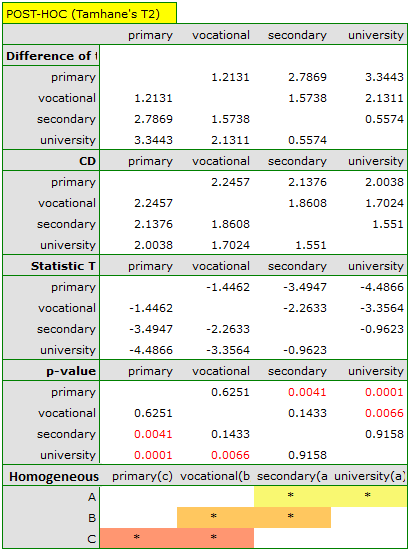
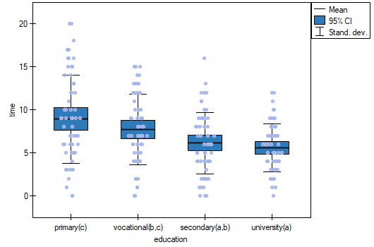
The least significant difference (LSD) determined for each pair of comparisons is not the same (even though the group sizes are equal) because the variances are not equal. Relating the LSD value to the resulting differences in mean values yields the same result as comparing the p-value with a significance level of $\alpha=0.05$ . The differences are between primary and higher education, primary and secondary education, and vocational and higher education. The resulting homogeneous groups overlap. In general, however, looking at the graph, we might expect that the more educated a person is, the less time it takes them to find a job.

In order to test the stated hypothesis, it is necessary to perform the trend analysis. To do so, we {reopen the analysis} with the button and, in the test options window, select: the Tamhane's T2 method, the Contrasts option (and set the appropriate contrast), or the For trend option (and indicate the order of education categories by specifying consecutive natural numbers).

Depending on whether the direction of the correlation between education and job search time is known to us, we use a one-sided or two-sided p-value. Both of these values are less than the given significance level. The trend we predicted is confirmed, that is, at a significance level of $\alpha=0.05$ we can say that this trend does indeed exist in the population from which the sample is drawn.

¹⁾

Brown M. B., Forsythe A. B. (1974), The small sample behavior of some statistics which test the equality of several means. Technometrics, 16, 385-389

²⁾

Welch B. L. (1951), On the comparison of several mean values: an alternative approach. Biometrika 38: 330–336

³⁾

Tamhane A. C. (1977), Multiple comparisons in model I One-Way ANOVA with unequal variances. Communications in Statistics, A6 (1), 15-32

⁴⁾

Brown M. B., Forsythe A. B. (1974), The ANOVA and multiple comparisons for data with heterogeneous variances. Biometrics, 30, 719-724

⁵⁾

Games P. A., Howell J. F. (1976), Pairwise multiple comparison procedures with unequal n's and/or variances: A Monte Carlo study. Journal of Educational Statistics, 1, 113-125

PQStat - Baza Wiedzy

Narzędzia użytkownika

Narzędzia witryny

Pasek boczny

The ANOVA for independent groups with F* and F" corrections

Narzędzia strony