PQStat - Baza Wiedzy

Local Getis-Ord’s G statistic

Getis and Ord's $G_i$ statistic (Getis and Ord 1992, Ord and Getis 1995) allows the detection of a local concentration of high and low values in neighboring objects and studies the statistical significance of that dependence. Getis and Ord have also defined a $G^*_i$ statistics, very similar to the $G_i$ statistics. The only difference between them is that in the case of the former the object for which the study is made also takes part in the analysis. In a weight matrix, then, the so-called potential is defined for that object, i.e. the neighborhood with itself (values on the axis are greater than 0).

Getis-Ord’s G coefficient

The local form of Getis and Ord's $G$ coefficient for the $i$ observation is defined with the formula:

$\begin{displaymath} G_i=\frac{\sum_{j=1}^nw_{ij}x_j}{\sum_{j=1}^nx_j}, \quad \textrm{where: $i\neq j$.} \end{displaymath}$

The $G^*_i$ coefficient is defined with the same formula but the computations are also made for the studied object, that is the object for which the $i$ and the $j$ indexes are equal.

As the coefficient is based on a quotient of two sums of the values of the ( $x_j$ ) objects, in order to interpret the coefficient correctly it is important that the analyzed phenomenon is described with the use of positive numbers. The interpretation of Getis and Ord's local coefficient, similarly to local Moran's coefficient, depends, to a great degree, on the selected weight matrix (row standardization of the matrix is recommended). High values of the $G_i$ or $G^*_i$ coefficients point to a concentration of objects with high values of the analyzed phenomenon, whereas low values point to a clustering of objects with low values. When the values are close to the expected value then the spatial distribution of the studied value is random.

The expected value is defined with the formula:

$\begin{displaymath} E(G_i)=\frac{\sum_{j=1}^nw_{ij}}{n-1}, \quad \textrm{where: $i\neq j$}; \end{displaymath}$

$\begin{displaymath} E(G_i^*)=\frac{\sum_{j=1}^nw_{ij}}{n}. \end{displaymath}$

The significance of Getis and Ord's coefficient

By testing the statistical significance of the relationship among the neighboring objects the following hypotheses are studied:

$\begin{array}{clccl} \mathcal{H}_0: & G_i = E(G_i) & \quad & \mathcal{H}_0: & G_i^* = E(G_i^*)\\ \mathcal{H}_1: & G_i \ne E(G_i), & \quad & \mathcal{H}_1: & G_i^* \ne E(G_i^*). \end{array}$

The test statistic has the form presented below:

$\begin{displaymath} Z_i(G)=\frac{\sum_{j=1}^nw_{ij}x_j-\overline{x}(i)\sum_{j=1}^nw_{ij}}{s(i)\sqrt{\frac{(n-1)\sum_{j=1}^nw_{ij}^2-\left(\sum_{j=1}^nw_{ij}\right)^2}{n-2}}}, \quad \textrm{where: $i\neq j$}; \end{displaymath}$

$\begin{displaymath} Z_i(G*)=\frac{\sum_{j=1}^nw_{ij}x_j-\overline{x}^*\sum_{j=1}^nw_{ij}}{s^*\sqrt{\frac{n\sum_{j=1}^nw_{ij}^2-\left(\sum_{j=1}^nw_{ij}\right)^2}{n-1}}}. \end{displaymath}$

where:

$\overline{x}(i)$ i $\overline{x}^*$ – the mean of the variable $X$ ,

$s(i)^2$ i $s^{*2}$ – the variance of the $X$ variable.

The $Z_i$ statistics has, asymptotically (for large sample sizes), normal distribution.

The p-value, designated on the basis of the test statistic, is compared with the significance level $\alpha$ :

$\begin{array}{ccl} $ if $ p \le \alpha & \Longrightarrow & $ reject $ \mathcal{H}_0 $ and accept $ \mathcal{H}_1, \\ $ if $ p > \alpha & \Longrightarrow & $ there is no reason to reject $ \mathcal{H}_0. \\ \end{array}$

Due to the problem of a lack of independence of coefficients computed for neighboring objects it is suggested to use a corrected significance level $\alpha$ . The suggested corrections are: Bonferroni correction: $\alpha_1=\alpha/k$ or Šidák correction: $\alpha_1=1-(1-\alpha)^{1/k}$ , where $k$ is the arithmetic mean number of the neighbors.

Map layers

The combination of the information from the value of the $Z_i$ statistic and its significance presents the so-called spacial regimes on the map:

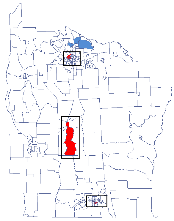
Statistically significant objects with high values of the $Z_i$ statistic are marked as High-High (objects with high values surrounded by objects with high values) and marked in red on the map;
Statistically significant objects with low values of the $Z_i$ statistic are marked as Low-Low (objects with low values surrounded by objects with low values) and marked in blue on the map;

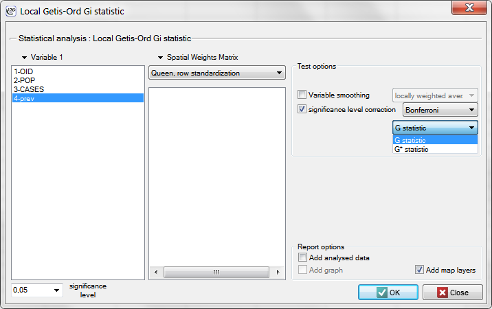
The window with settings for Local Getis and Ord's analysis is accessed via the menu Spatial analysis → Spatial statistics → Getis-Ord <latex>$G_i$</latex> statistic.

EXAMPLE con. (catalog: leukemia, file: leukemia)

We will analyze the data concerning leukemia.

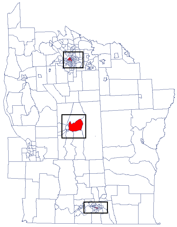
The map leukemia contains information about the location of 281 polygons (census tracts) in the northern part of the state of New York.
Data for the map leukemia:
- Column CASES – the number of cases of leukemia in the years 1978-1982, ascribed to particular objects (census tracts). The value should be an integral number, however, in agreement with Waller's (1994) description, some cases which could not be objectively ascribed to a particular region have been divided proportionately. Hence, the numerousnesses of the cases ascribed to the 281 objects are not integral numbers.
- Column POP – population size in particular objects.
- Column prev – the frequency coefficient of leukemia per 100000 people, for each object in one year: prev=(CASES/POP)*100000/5

The global analysis has not yielded an unambiguous answer as to the occurrence of spatial autocorrelation. We will, then, check if we can find regions in which the prevalence of leukemia is significantly higher.

In order to localize leukemia clusters we will compute the $G_i$ and $G_i^*$ coefficients. The analysis will be conducted with the prev variable and the neighborhood matrix – Queen, row standardized (according to contiguity) which is suggested by the program. In order to use a different matrix one has to generate it first, see chapter: Spatial weight matrix. We also select one of the corrections of the significance level.

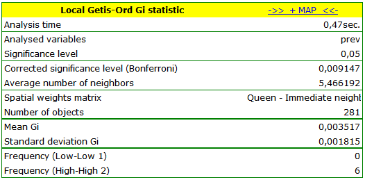
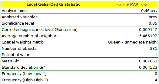
The obtained report presents the values of local coefficients, the values of test statistics, and the corresponding values of test probability. We will also find the information about the number of regions defining the spatial regimes (High-High, Low-Low). Also, a result is ascribed to the analysis, which we can draw on the map (button ) – those spatial regimes are defined in the report with the use of the color column.

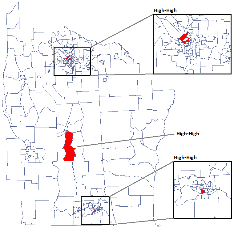
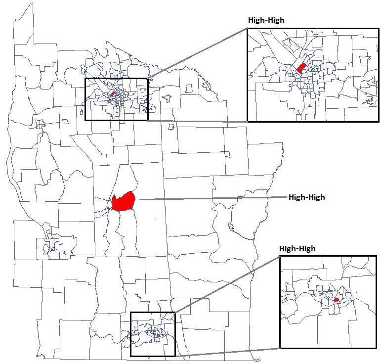
We were able to localize 3 clusters (6 census tracts in the analysis of the $G_i$ coefficient and 4 tracts in the analysis of the $G_i^*$ coefficient) in which the prevalence of leukemia is significantly higher. They are the centers of clusters with high values of leukemia, marked in red on the map.

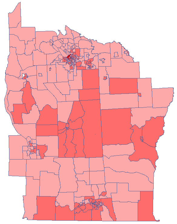
The obtained results can be additionally illustrated by coloring the map so as to present the values of the local Getis and Ord's coefficient or the values of the test statistic, or the $p$ values. One just has to copy the appropriate columns from the report and paste them into a datasheet. In this example we will use the values of the $Z(G_i)$ test statistic for coloring. Having pasted it into an empty column of a datasheet, in the map manager we color the base map according to the values of that column, selecting the standard deviation with the coefficient 3 as a way of gradiating colors. Positive and high values of the $Z_i$ statistic point to a concentration of objects with high values, whereas negative and low values point to a concentration of objects with low values, and the values near zero point to a random spatial distribution of the studied variable (a map can be added with means and confidence intervals).

By analyzing the smoothed variable textsf{prev} we strengthen the clusterization effect. We obtain a similar result, i.e. 3 clusters (15 census tracts in the analysis of the $G_i$ coefficient and 9 tracts in the analysis of the $G_i^*$ coefficient) which are cluster centers.

PQStat - Baza Wiedzy

Narzędzia użytkownika

Narzędzia witryny

Pasek boczny

Local Getis-Ord’s G statistic

Narzędzia strony