PQStat - Baza Wiedzy

Local Moran's I statistic

Local Moran's I statistic is the most popular analysis from those defined as LISA (Local Indicators of Spatial Association) (Luc Anselin 1995 ¹⁾. In contrast to Global Moran's I statistic it defines the local spacial autocorrelation, i.e. defines the similarity of a spatial unit to its neighbors and studies the statistical significance of that dependence.

Local Moran's I coefficient

The local form of Moran's $I$ coefficient for the $i$ observation is defined with the formula:

$\begin{displaymath} I_i=\frac{\left(x_i-\overline{x}\right)\sum_{j=1}^nw_{ij}\left(x_j-\overline{x}\right)}{\sigma^2} \end{displaymath}$

where:

$n$ – the number of spatial objects (the number of points or polygons),

$x_i$ , $x_j$ – are the values of the variable for the compared objects,

$\overline{x}$ – it is the mean value of the variable for all objects,

$w_{ij}$ – elements of a spacial weight matrix (it is recommended that the matrix is row standardized),

$\sigma^2=\frac{\sum_{i=1}^n\left(x_i-\overline{x}\right)^2}{n-1}$ – variance

The interpretation of the local Moran's coefficient is analogous to its global counterpart, however, it largely depends on the selected weight matrix. Most often non-zero matrices are ascribed only to neighboring objects. As a result the local coefficient only describes the similarity of objects in the zone of neighborhood. Row standardization makes it easier to compare the values of coefficients obtained for various objects as the expected value for each coefficient is then the same.

High values of a coefficient point to the occurrence of clusters with similar values while low values of a coefficient point to the occurrence of the so-called hot spots, and values near the expected value $E(I_i)$ point to the random distribution in space of the studied variable.

The expected value is defined with the formula:

$\begin{displaymath} E(I_i)=\frac{-\sum_{j=1}^nw_{ij}}{n-1} \end{displaymath}$

The significance of Moran's autocorrelation coefficient

By testing the statistical significance of the relationship among the neighboring objects the following hypotheses are studied:

$\begin{array}{cl} \mathcal{H}_0: & I_i = E(I_i), \\ \mathcal{H}_1: & I_i \ne E(I_i). \end{array}$

The test statistic has the form presented below:

$\begin{displaymath} Z_i=\frac{I_i-E(I_i)}{\sqrt{var(I_i)}}, \end{displaymath}$

where:

$\displaystyle var(I_i)=\frac{w_{i(2)}(n-b_2)}{n-1}+\frac{2w_{i(kh)}(2b_2-n)}{(n-1)(n-2)}-\frac{\left(\sum_{j=1}^nw_{ij}\right)^2}{(n-1)^2}$ – variance in a random distribution,

$b_2=\frac{(n-1)\sum_{i=1}^n\left(x_i-\overline{x}\right)^4}{\left(\sum_{i=1}^n\left(x_i-\overline{x}\right)^2\right)^2}$ ,

$w_{i(2)}$ – the sum of weights square for the $i$ row,

$2w_{i(kh)}$ – the sum of possible weights ratios for the $i$ row, after the exclusion of ratios with the same indexes.

The $Z_i$ statistics has, asymptotically (for large sample sizes), rnormal distribution.

The p-value, designated on the basis of the test statistic, is compared with the significance level $\alpha$ :

$\begin{array}{ccl} $ if $ p \le \alpha & \Longrightarrow & $ reject $ \mathcal{H}_0 $ and accept $ \mathcal{H}_1, \\ $ if $ p > \alpha & \Longrightarrow & $ there is no reason to reject $ \mathcal{H}_0. \\ \end{array}$

Due to the problem of a lack of independence of coefficients computed for neighboring objects it is suggested to use a corrected significance level $\alpha$ . The suggested corrections are: Bonferroni correction: $\alpha_1=\alpha/k$ or Šidák correction: $\alpha_1=1-(1-\alpha)^{1/k}$ , where $k$ is the arithmetic mean number of the neighbors.

Map layers

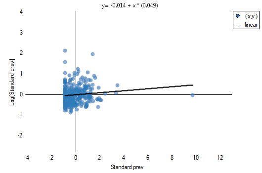
The combination of information from Moran's scatter plot (the division of objects into: High-High, Low-Low, Low-High, High-Low) and from the significance of the local Moran's statistics presents on a map the so-called spatial regimes:

Statistically significant High-High objects (objects with high values surrounded by objects with high values) are marked in red on the map;
Statistically significant Low-Low objects (objects with low values surrounded by objects with low values) are marked in blue on the map;
Statistically significant Low-High objects (objects with low values surrounded by objects with high values) are marked in light blue on the map;
Statistically significant High-Low objects (objects with high values surrounded by objects with low values) are marked in light red on the map.

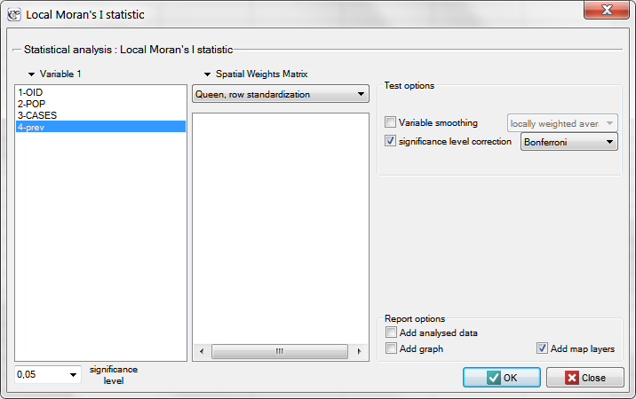
The window with the settings of the local Moran's analysis option is accessed via the menu Spatial analysis → Spatial statistics → Local Moran's I statistic.

EXAMPLE cont. (catalog: leukemia, file: leukemia)

We will analyze data about leukemia.

The map leukemia contains information about the location of 281 polygons (census tracts) in the northern part of the state of New York.
Data for the map leukemia:
- Column CASES – the number of cases of leukemia in the years 1978-1982, ascribed to particular objects (census tracts). The value should be an integral number, however, in agreement with Waller's (1994) description, some cases which could not be objectively ascribed to a particular region have been divided proportionately. Hence, the numerousnesses of the cases ascribed to the 281 objects are not integral numbers.
- Column POP – population size in particular objects.
- Column prev – the frequency coefficient of leukemia per 100000 people, for each object in one year: prev=(CASES/POP)*100000/5

The global analysis has not yielded an unambiguous answer as to the occurrence of spatial autocorrelation. We will, then, check if we can find regions in which the prevalence of leukemia is significantly higher.

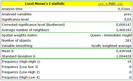
In order to localize clusters of leukemia and regions which contrast with the environment with respect to the prevalence of that disease we will compute the local Moran's coefficient. For the analysis we will use the prev variable and the neighborhood matrix – Queen, row standardized (according to the contiguity) which is suggested by the program. In order to use a different matrix one has to generate it first, see chapter: Spatial weight matrix. We also select one of the corrections of the significance level.

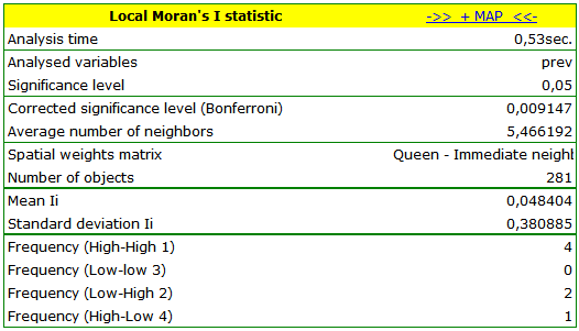
The obtained report presents the values of local coefficients, the values of test statistics, and the corresponding values of test probability. We will also find here the information about the number of regions defining the spatial regimes (High-High, Low-Low, Low-High, High-Low).

Also, a result is ascribed to the analysis, which we can draw on the map (button ) – those are spatial regimes described in the report with the use of the color column.

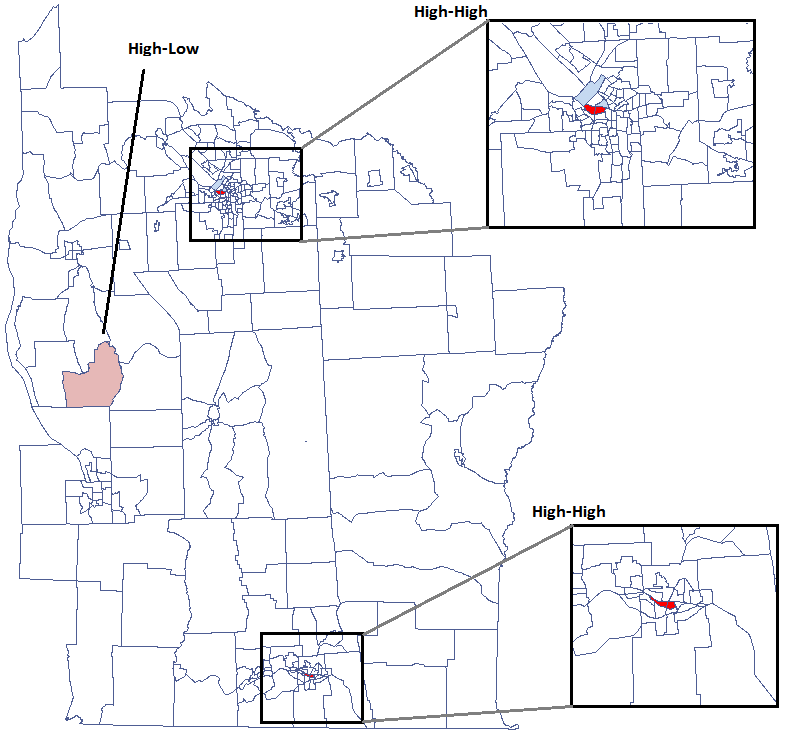
We have been able to localize small but significant clusters in which the prevalence of leukemia is higher. The red color is used for the 2 clusters (4 register regions) lying in smaller and more populated regions – they are the centers of the clusters with high leukemia values. The light red color is used for the census tract with high values of the coefficient describing the prevalence of leukemia. The region contrasts with the neighboring census tracts which are characterized by a relatively low coefficient.

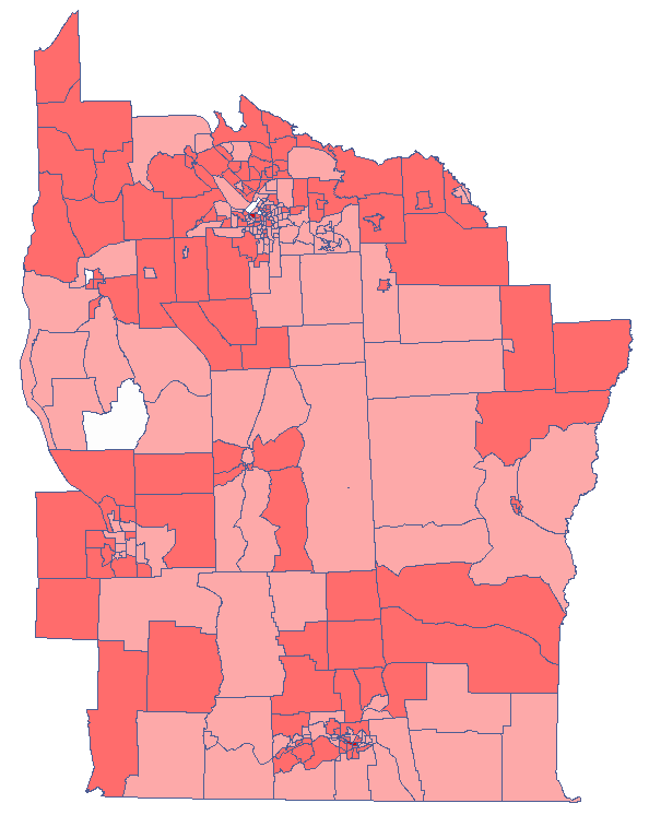
The obtained results can be further illustrated when the map is colored with the values of the local Moran's $I_i$ coefficient or the values of a test statistic, or $p$ values. One just has to copy the appropriate columns from the report into a datasheet. In this example we will use the values of the $Z(I_i)$ test statistic for coloring. Having pasted it into an empty column of a datasheet, in the map manager we color the base map according to the values of that column, selecting the standard deviation with the coefficient 3 as a way of gradiating colors. Positive and high values of the $Z_i$ statistics point to the occurrence of clusters of similar values while negative and low values of that statistic point to the occurrence of the so-called hot spots. Values close to 0 point to a random distribution of the studied value in space.

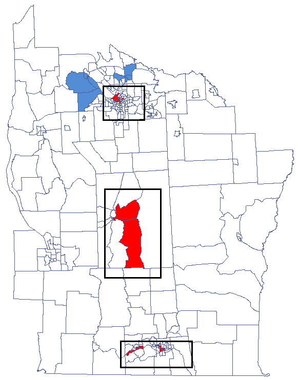
By analyzing the smoothed variable prev we strengthen the clusterization effect. We obtain a similar result but this time we localize 3 clusters (19 census tracts) which are cluster centers.

¹⁾

Anselin L. (1995), Local Indicators of Spatial Association – LISA; Geographical Analysis, 27(2): 93–115

PQStat - Baza Wiedzy

Narzędzia użytkownika

Narzędzia witryny

Pasek boczny

Local Moran's I statistic

Narzędzia strony