PQStat - Baza Wiedzy

Quadrat Count Methods

Graphically, this method is a generalization of a histogram, or one-dimensional analysis, to a two-dimensional case. Building a histogram we have one variable, which we divide into intervals of equal length and give the number of cases in each interval. When building a grid of squares, we have two variables on which we build the grid and give the number of cases in each grid square (DPS – Dot Per Square). The ratio of this number to the area of a square determines the intensity of the color in which a given grid square is colored.

$\begin{tabular}{|l|l|l|l|} \hline \cellcolor[rgb]{0.8,0.8,0.8}&\textcolor[rgb]{1,1,1}{aaa}&\cellcolor[rgb]{0.4,0.4,0.4}\textcolor[rgb]{0.4,0.4,0.4}{aa}$\bullet$&\textcolor[rgb]{1,1,1}{aaa}\\ \cellcolor[rgb]{0.8,0.8,0.8}$\bullet$&&\cellcolor[rgb]{0.4,0.4,0.4}$\bullet$&\\ \hline \textcolor[rgb]{1,1,1}{aaa}&\textcolor[rgb]{1,1,1}{aaa}&\textcolor[rgb]{1,1,1}{aaa}&\textcolor[rgb]{0.8,0.8,0.8}{aa}\cellcolor[rgb]{0.8,0.8,0.8}$\bullet$\\ \textcolor[rgb]{1,1,1}{aaa}&\textcolor[rgb]{1,1,1}{aaa}&\textcolor[rgb]{1,1,1}{aaa}&\cellcolor[rgb]{0.8,0.8,0.8}\\ \hline \end{tabular}$

Based on the number of casess in the grid squares, we can study their spatial distribution. If there are the same number of points in each square, it means perfectly uniform distribution. When the opposite is true, when the variation in the number of points in the squares is very large, it means that there are squares with a much larger number of points, that is, clusters are formed.

If we denote by $n$ the number of points of the study area and by $m$ the number of squares into which the study area is divided, then we can determine the mean, variance, and standard deviation of the number of points per square:

$\begin{displaymath} \overline{DPS}=\frac{n}{m}, \quad Var_{(DPS)}=\frac{\sum_{i=1}^k m_i(n_i-\mu)^2}{m -1}, \quad SD_{(DPS)}=\sqrt{var}, \end{displaymath}$

where $m_i$ – is the number of squares with the number of points equal to $n_i$ .

Coefficient $VMR_{(DPS)}$

The most important information is provided by the variance-mean ratio – the coefficient, which is the quotient of the variance and the mean:

$\begin{displaymath} VMR_{(DPS)}=\frac{Var}{\overline{DPS}} \end{displaymath}$

A value of $VMR_{(DPS)}<1$ indicates too little variation in the number of points in squares which suggests a uniform dispersion effect, $VMR_{(DPS)}>1$ indicates too much variation in the number of points in squares and therefore a clustering effect, and a value close to 1 indicates an average variation in the number of points in squares which implies a random distribution of points.

The Index of Cluster Size (ICS) is often considered in the literature:

$\begin{displaymath} ICS_{(DPS)}=VMR_{(DPS)}-1 \end{displaymath}$ The expected value of $ICS_{(DPS)}$ assuming random points is 0. A positive value indicates a clustering effect and a negative value indicates a regular distribution of points.

Significance of the coefficient $VMR_{(DPS)}$

The $VMR_{(DPS)}$ coefficient significance test is used to verify the hypothesis that the observed point counts n the squares are the same as the expected counts that would occur for a random distribution of points.

Hypotheses:

$\begin{array}{ll} \mathcal{H}_0: & VMR_{(DPS)}=1,\\ \mathcal{H}_1: & VMR_{(DPS)} \neq 1. \end{array}$

The test statistic has the form:

$\begin{displaymath} \chi^2=(m-1)\cdot VMR_{(DPS)}. \end{displaymath}$

This statistic has an asymptotically $\chi^2$ distribution with $df=m-1$ degrees of freedom.

The p-value, designated on the basis of the test statistic, is compared with the significance level $\alpha$ :

$\begin{array}{ccl} $ if $ p \le \alpha & \Longrightarrow & $ reject $ \mathcal{H}_0 $ and accept $ \mathcal{H}_1, \\ $ if $ p > \alpha & \Longrightarrow & $ there is no reason to reject $ \mathcal{H}_0. \\ \end{array}$

Note

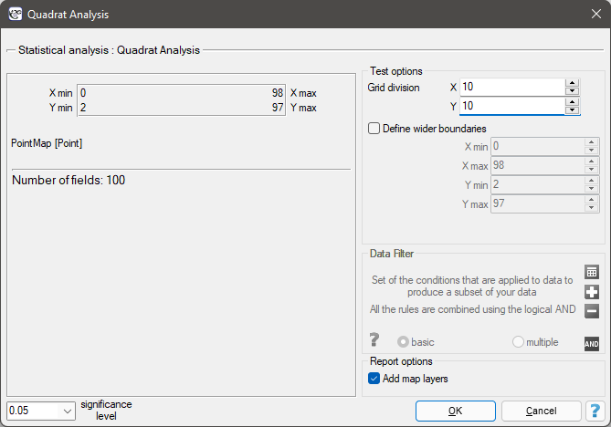
The result of the analysis depends to a large extent on the density of the grid and thus on the number/size of squares into which the analyzed area is divided. In the test options window, you can set the grid that will be used to divide the test area into squares by specifying the number of squares vertically and horizontally.

The window with the settings for the quadrat count method is launched via the menu Spatial Analysis→Spatial Statistics→Quadrat analysis

EXAMPLE (file squares.pqs)

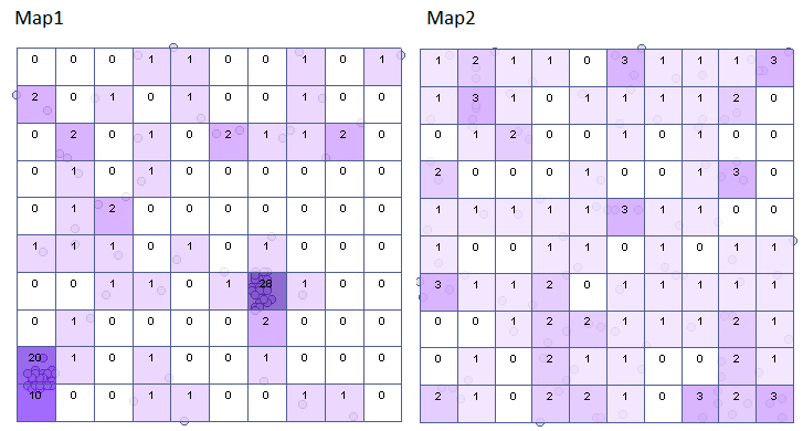
Using the datasheet, generate two point maps and perform a density analysis of these points. Answer the question: are the points randomly distributed in each of these maps?

You create the point maps using the formulas: menu Data→Formulas…

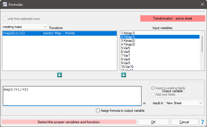
This will result in two new sheets containing maps. For each of these sheets, we perform a quadrat analysis.

Hypotheses:

$\begin{array}{ll} \mathcal{H}_0: & $the distribution of points in the population from which the sample is drawn is random ,$\\ \mathcal{H}_1: & $the distribution of points in the population from which the sample is drawn is not random.$ \end{array}$

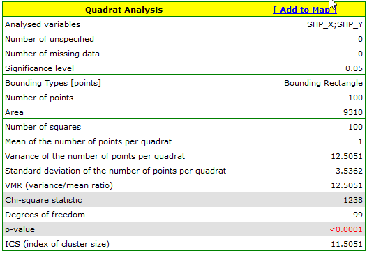
The results for Map 1 indicate a significant variation in the number of points in the squares, that is, a clustering effect (value p=<0.0001). This effect persists for different grid densities. For a grid density of 10:10 the VMR ratio is as high as 12.5, the entire report is included below:

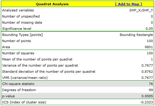
For map 2, the situation is quite different. For the 10:10 density grid, we have a lack of statistical significance (value p=0.9585) and the value of the coefficient VMR=0.77 indicate that the distribution of points is random.

Using the 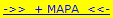button in the report, we move to the Map Manager to select the analysis grid from the displayed list of layers and obtain a graphic interpretation of the results.

PQStat - Baza Wiedzy

Narzędzia użytkownika

Narzędzia witryny

Pasek boczny

Quadrat Count Methods

Narzędzia strony