PQStat - Baza Wiedzy

Spis treści

Kernel density estimator
- Two-dimensional kernel estimator
- Three-dimensional kernel estimator

Kernel density estimator

Two-dimensional kernel estimator

The two-dimensional kernel estimator (like the one-dimensional estimator) allows the distribution of the data, expressed by the method of squares, to be approximated by smoothing.

The two-dimensional kernel density estimator approximates the density of a data distribution by creating a smoothed density plane in a non-parametric manner. It produces a better density estimate than is given by the traditional method of squares, whose squares form a step function.

As in the one-dimensional case, this estimator is defined based on appropriately smoothed summed kernel functions (see description in the PQStat User Manual). There are several smoothing methods to choose from and several kernel functions described for the one-dimensional estimator (Gaussian, uniform, triangular, Epanechnikov, quartic/biweight). While the kernel function has little effect on the resulting plane smoothing, the smoothing factor does.

For each point $x$ in the range defined by the data, the density or kernel estimator is determined. It is obtained by summing the product of the kernel function values at that point:

$\begin{displaymath} \hat{f}_K(x,y)=\frac{1}{n}\sum_{i=1}^nK_h(t_i)K_h(s_i) \end{displaymath}$

If we give the individual cases weights $w_i$ , then we can construct a weighted nuclear density estimator defined by the formula:

$\begin{displaymath} \hat{f}_K(x,y)=\frac{1}{\sum_{i=1}^nw_i}\sum_{i=1}^nw_iK_h(t_i)K_h(s_i) \end{displaymath}$

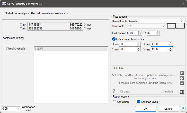
The window with settings for the kernel 2D density estimator ptions is launched via the menu Spatial analysis→Spatial statistics→Kernel density estimator 2D

EXAMPLE (snow.pqs plik)

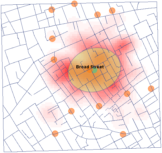
Currently, the main problem in presenting point data on the location of people is the need to protect them. Data protection prohibits publishing research results in such a way, that it would be possible to recognize a given person on their basis. A good solution in this case is a point density estimator.

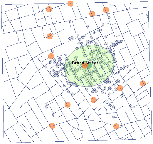
We will present point data illustrating the cholera epidemic in London in 1854 using such an estimator. To do so, we will use a map of points (deaths due to cholera) with layers already overlaid to illustrate both streets and water pumps, and the result of an analysis by physician John Snow.

In the analysis window for the point map, we will stay with the Gaussian (normal) distribution kernel and the SNR smoothing factor. The grid density will be set to 80:80 and the boundaries will be increased so that the edges do not have a sharp edge by entering 300 as the minimum value for the X and Y coordinates and 1100 as the maximum value.

Using the 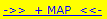button in the report, we go to the Map Manager, where we can add a layer representing this estimator (the last item in the list of layers).

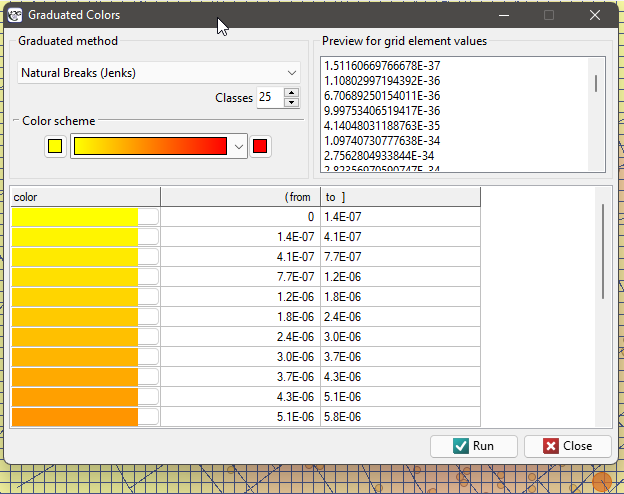
After applying the nuclear density estimator layer, edit it o remove the grid lines and change the yellow color to the natural background color (white in this case). The layer thus obtained is moved up g_kolejnosc_warstw, so that it is drawn at the beginning. We turn off the points layer (Base Map).

EXAMPLE cont. (squares.pqs file)

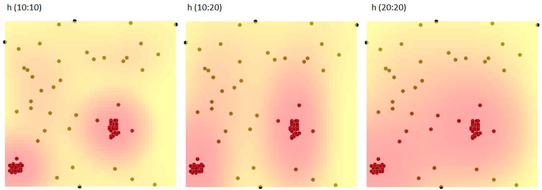
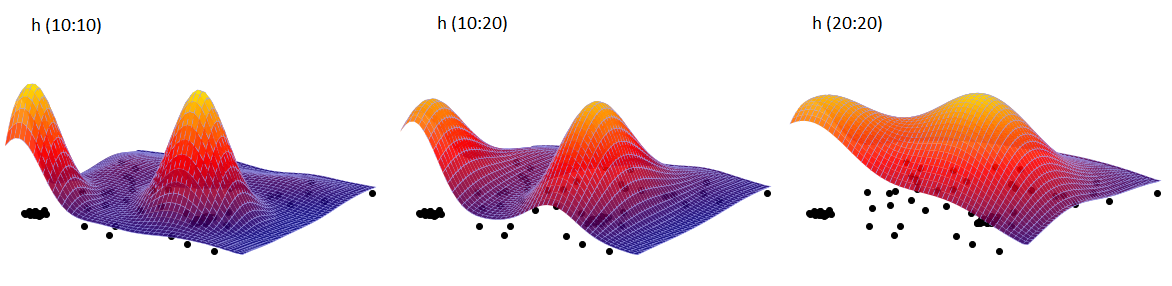
Using the kernel estimator, we represent the point density for map 1 - obtained in the earlier part of the task.

In the analysis window, we set the grid density to 50:50 and the kernel type as normal distribution and include a graph. We perform the analysis three times while changing the User smoothing factor: h (10:10), then h (10:20) and h (20:20). The obtained results presented on the map (via Map Manager) and on the 3D graph are shown below:

Three-dimensional kernel estimator

The three-dimensional kernel estimator (like the one-dimensional estimator and the two-dimensional estimator) allows you to approximate the distribution of the data by smoothing it.

The three-dimensional kernel density estimator approximates the density of the data distribution by creating a smoothed density plane in a non-parametric way. Graphically, we can represent it by plotting the first two dimensions in layers created by the third dimension. As in the one-dimensional case (see description in the PQStat User's Guide) and the two-dimensional estimator, this estimator is defined based on appropriately smoothed summed kernel functions. There are several smoothing methods to choose from and several kernel functions described for the one-dimensional estimator (Gaussian, uniform, triangular, Epanechnikov, quartic/biweight). While the kernel function has little effect on the resulting plane smoothing, the smoothing factor does.

For each point $x$ in the range defined by the data, the density that is the kernel estimator is determined. It is formed by summing the product of the kernel function values at that point:

$\begin{displaymath} \hat{f}_K(x,y,z)=\frac{1}{n}\sum_{i=1}^nK_h(t_i)K_h(s_i)K_h(r_i) \end{displaymath}$

If we give the individual cases weights $w_i$ , then we can construct a weighted kernel density estimator defined by the formula:

$\begin{displaymath} \hat{f}_K(x,y,z)=\frac{1}{\sum_{i=1}^nw_i}\sum_{i=1}^nw_iK_h(t_i)K_h(s_i)K_h(r_i) \end{displaymath}$

The window with settings for the kernel 3D density estimator options is launched via the menu Spatial analysis→Spatial statistics→Kernel 3D density estimator

Note

Displaying subsequent layers of the estimator, determined by the third dimension, is possible by editing the layer in the map Manager window and selecting the appropriate layer index.

PQStat - Baza Wiedzy

Narzędzia użytkownika

Narzędzia witryny

Pasek boczny

Spis treści

Kernel density estimator

Two-dimensional kernel estimator

Three-dimensional kernel estimator

Narzędzia strony