PQStat - Baza Wiedzy

Global Geary's C statistic

Similarly to Moran's analysis, global Geary's statistic studies the degree of the intensity of a given feature in spatial objects.

Note

It is not recommended to conduct Geary's analysis for objects without a neighborhood (objects described in a weight matrix only with the value 0). Such objects can be excluded from the analysis by deactivating them (Chapter Limiting the workspace), or the analysis can be made with the use of a different manner of defining neighborhood (a different weight matrix).

Geary's autocorrelation coefficient – introduced by Geary in 1954 ¹⁾.

It is one of the possible alternatives for the global Moran's statistic. Similarly to Moran's analysis, Geary's statistic studies the degree of intensity of a given $x_i$ feature in spatial objects described with the use of a weight matrix with $w_{ij}$ elements. This time, instead of computing the sum of quotients:

$\sum\sum w_{ij}(x_i-\overline{x})(x_j-\overline{x})$

we compute the sum of the difference squares:

$\begin{displaymath} \sum\sum w_{ij}(x_i-x_j)^2 \end{displaymath}$

As a result, Geary's autocorrelation coefficient is expressed with the formula:

$\begin{displaymath} c=\frac{\sum_{i=1}^n\sum_{j=1}^nw_{ij}(x_i-x_j)^2}{2 S_0 sd^2} \end{displaymath}$

where:

$n$ – the number of spatial objects (the number of points or polygons),

$x_i$ , $x_j$ – are the values of the variable for the compared objects,

$w_{ij}$ – elements of the spatial weights matrix (weights matrix row standardized),

$S_0=\sum_{i=1}^n\sum_{j=1}^nw_{ij}$ ,

$sd^2=\frac{\sum_{i=1}^n\left(x_i-\overline{x}\right)^2}{n-1}$ – variance,

$\overline{x}$ – it is the mean value of the variable for all objects.

The interpretation of Geary's coefficient:

$c<1$ and $c \approx 0$ means the occurrence of clusters with similar values – a positive autocorrelation;
$c>1$ means the occurrence of the so-called hot spots, i.e. distinctly different values in neighboring areas – a negative autocorrelation;
$c \approx 1$ means a random spatial distribution of the studied variable – a lack of autocorrelation.

Note

When the values of a studied feature are characterized by a great variability of variance then it is desirable to stabilize that variability. The basic information about smoothing variables have been described in the Chapter \ref{wygladz_przestrz} SPATIAL SMOOTHING

Significance of Geary's autocorrelation coefficient

A test for checking the significance of Geary's autocorrelation coefficient serves the purpose of verifying the hypothesis about a lack of spatial autocorrelation

Hypotheses:

$\begin{array}{cl} \mathcal{H}_0: & C = 1, \\ \mathcal{H}_1: & C \ne 1. \end{array}$

The test statistic has the form presented below:

$\begin{displaymath} Z=\frac{C-E(C)}{\sqrt{var(C)}}, \end{displaymath}$

where:

$\displaystyle E(C)=1$ – the expected value,

$\displaystyle var(C)$ – variance.

Depending on the assumption concerning the distribution of the population from which the sample has been taken, the manner of selecting variance is chosen (Cliff and Ord (1981)²⁾, and Goodchild (1986)³⁾). If it is a normal distribution, then:

$\begin{displaymath} var(C)=\frac{(2S_1+S_2)(n-1)-4S_0^2}{2(n+1)S_0^2}, \end{displaymath}$

where:

$S_1$ and $S_2$ are defined as for Moran's analysis.

If it is a random distribution, then:

$var(CS)=\frac{(n-1)S_1\left(n^2-3n+3-(n-1)b_2\right)-(n-1)S_2\left(n^2+3n-6-(n^2-n+2)b_2\right)\frac{1}{4}+S_0^2\left(n^2-3-(n-1)^2b_2\right)}{n(n-2)^{(2)}S_0^2},$

where:

$b_2=\frac{\frac{1}{n}\sum_{i=1}^n\left(x_i-\overline{x}\right)^4}{\left(\frac{1}{n}\sum_{i=1}^n\left(x_i-\overline{x}\right)^2\right)^2}$ ,

$n^{(b)}=n(n-1)(n-2)...(n-b+1)$ .

Statistics $Z$ has, asymptotically (for large sample sizes), normal distribution.

The p-value, designated on the basis of the test statistic, is compared with the significance level $\alpha$ :

$\begin{array}{ccl} $ if $ p \le \alpha & \Longrightarrow & $ reject $ \mathcal{H}_0 $ and accept $ \mathcal{H}_1, \\ $ if $ p > \alpha & \Longrightarrow & $ there is no reason to reject $ \mathcal{H}_0. \\ \end{array}$

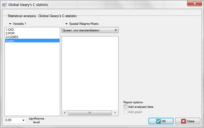
The window with settings for Geary's analysis is accessed via the men Spacial analysis → Spacial statistics → Global Geary's C statistic.

EXAMPLE cont. (catalog: leukemia, file: leukemia)

We will analyze the data concerning leukemia.

The map leukemia contains information about the location of 281 polygons (census tracts) in the northern part of the state of New York.
Data for the map leukemia:
- Column CASES – the number of cases of leukemia in the years 1978-1982, ascribed to particular objects (census tracts). The value should be an integral number, however, in agreement with Waller's (1994) description, some cases which could not be objectively ascribed to a particular region have been divided proportionately. Hence, the numerousnesses of the cases ascribed to the 281 objects are not integral numbers.
- Column POP – population size in particular objects.
- Column prev – the frequency coefficient of leukemia per 100000 people, for each object in one year: prev=(CASES/POP)*100000/5

Global Moran's analysis has pointed to a lack of spatial autocorrelation. This time, in order to check if in the studied area of the northern part of the state of New York it is possible to localize clusters of leukemia we will compute the global Geary's C statistic.

We start from the presentation of the geographic distribution of the prevalence coefficient (prev) on the map, according to the values of the prev variable, dividing it into quartiles:

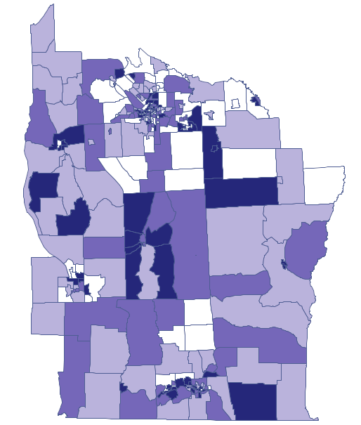
Dark colors on the map present the places with a higher prevalence of leukemia, whereas light places signify a lower prevalence. Geary's correlation coefficient obtained in the analysis equals: 0.884986.

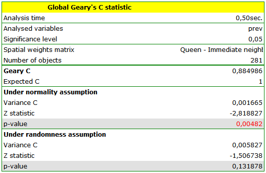
The obtained result, assuming a random distribution of data, is different from the result obtained with the assumption of a normal distribution. That can be indicative of an instability of the results and point to the need of further analyses based on smoothed variables.

¹⁾

Geary R.C. (1954), The Contiguity Ratio and Statistical Mapping. The Incorporated Statistician, 5, 115-45

²⁾

Cliff A.D., Ord J.K. (1981), Spatial Processes: Models and Applications. Pion: London

³⁾

Goodchild M.F. (1986), Spatial Autocorrelation, CATMOG 47, Geobooks: Norwich UK

PQStat - Baza Wiedzy

Narzędzia użytkownika

Narzędzia witryny

Pasek boczny

Global Geary's C statistic

Narzędzia strony