PQStat - Baza Wiedzy

Asymmetry testing

Symmetry in the effects obtained is usually indicative of the absence of publication bias, but it should be kept in mind that many objective factors can disrupt symmetry, e.g., studies with statistically insignificant effects or small studies are often not published, making it much more difficult to reach such results. At the same time, there are no sufficiently comprehensive and universal statistical tools for asymmetry detection. As a result, a significant part of meta-analyses is published despite the diagnosed asymmetry. Such studies, however, require good justification of such a procedure.

Funnel plot

$\begin{pspicture}(-1,-0.5)(7,5) \psline{->}(0,0)(0,4) \psline{->}(0,0)(5,0) \psdots(0.5,0.5) \psdots(1,1) \psdots(1.5,0.5) \psdots(1.5,2) \psdots(1.6,1.1) \psdots(1.8,2.4) \psdots(2,2) \psdots(2,2.8) \psdots(2.1,0.6) \psdots(2.5,4) \psdots(2.5,1.2) \psdots(2.5,2) \psdots(2.5,3) \psdots(2.5,4) \psdots(3,2.6) \psdots(2.8,3.1) \psdots(3,2) \psdots(2,1.3) \psdots(1.5,1.6) \psdots(3.3,2.2) \psellipse[linestyle=dashed,linecolor=red, dash=3pt 2pt](3.5,1)(-0.9,-0.9) \rput(3.5,1){\scriptsize bias} \rput(5.5,1.9){\scriptsize publication bias} \rput(5.9,1.3){\scriptsize asymmetrical plot} \rput(6.5,1.6){\tiny no studies in the bottom right corner of the plot} \end{pspicture}$

A standard way to test for publication bias in the form of asymmetry is a funnel plot, showing the relations between study size (Y axis) and summary effect size (X axis). It is assumed that large studies (placed at the top of the graph) in a correctly selected set, are located close together and define the center of the funnel, while smaller studies are located lower and are more diverse and symmetrically distributed. Instead of the study size on the Y-axis, the effect error for a given study can be shown, which is better than showing the study size alone. This is because the effect error is a measure that indicates the precision of the study and also carries information about its size.

Egger's test

Since the interpretation of a funnel plot is always subjective, it may be helpful to use the Egger coefficient (Egger 1997¹⁾), the interception of the fitted regression line. This coefficient is based on the correlation between the inverse of the standard error and the ratio of the effect size to its error. The further away from 0 the value of the coefficient, the greater the asymmetry. The direction of the coefficient determines the type of asymmetry: a positive value along with a positive confidence interval for it indicates an effect size that is too high in small studies and a negative value along with a negative confidence interval indicates an effect size that is too low in small studies.

Note

Egger's test should only be used when there is a large variation in study sizes and the occurrence of a medium-sized study.

Note

With few studies (small number of $k$ ), it is difficult to reach a significant result despite the apparent asymmetry.

Hypotheses:

$\begin{array}{cl} \mathcal{H}_0: & b = 0,\\ \mathcal{H}_1: & b \ne 0, \end{array}$

where:

$b$ – intercept in Egger's regression equation.

The test statistic is in the form of:

$\begin{displaymath} t=\frac{b}{SE(b)} \end{displaymath}$

where:

$SE(b)$ – standard error of intercept.

The test statistic has t-Student distribution with $k-2$ degrees of freedom.

The p value, designated on the basis of the test statistic, is compared with the significance level $\alpha$ :

$\begin{array}{ccl} $ if $ p \le \alpha & \Longrightarrow & $ reject $ \mathcal{H}_0 $ and accept $ \mathcal{H}_1, \\ $ if $ p > \alpha & \Longrightarrow & $ there is no reason to reject $ \mathcal{H}_0. \\ \end{array}$

Testing the „Fail-safe” number

Rosenthal’s Nfs - The „fail-safe” number described by Rosenthal (1979)²⁾ specifies the number of papers not indicating an effect (e.g., difference in means equal to 0, odds ratio equal to 1, etc.) that is needed to reduce the overall effect from statistically significant to statistically insignificant.

$\begin{displaymath} Nfs=\frac{\left(\sum_{i=1}^{k}Z_i\right)^2}{Z_c^2}-k \end{displaymath}$

where:

$Z_i$ – the value of the test statistic (with normal distribution) of a given test,

$Z_c$ – the critical value of the normal distribution for a given level of significance,

$k$ – number of studies in the meta-analysis.

Rosenthal (1984)³⁾ defined the number of papers being the cutoff point as $5k+10$ . By determining the quotient of $Nfs$ and the cutoff point, we obtain coefficient(fs). According to Rosenthal's interpretation, if coefficient(fs) is greater than 1, the probability of publication bias is minimal.

Orwin's Nfs - the „fail-safe” number described by Orwin (1983) determines the number of papers with the average effect indicated by the researcher $\overline{M_{fs}}$ that is needed to reduce the overall effect to the desired size $M_d$ indicated by the researcher.

$\begin{displaymath} Nfs=k\frac{M - M_d}{M_d-\overline{M_{fs}}} \end{displaymath}$

where:

$M$ – the overall effect obtained in the meta-analysis.

EXAMPLE cont (MetaAnalysisRR.pqs file)

When examining the effect of cigarette smoking on the onset of disease X, the assumption of study asymmetry, and therefore publication bias, was checked. To do this, the option Asymmetry was selected in the analysis window and Funnel plot was selected.

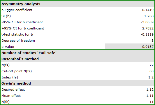
Egger's test result are not statistically significant (p=0.9137), indicating no publication bias.

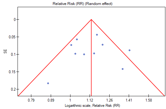
The points representing each study are symmetrically distributed in the funnel plot. Admittedly, one study is outside the boundary of the triangle (Study 3), but it is close to its edges. On the basis of the diagram we also have no fundamental objections to the choice of studies, the only concern being the third study.

The number of „fail-safe” papers determined by Rosenthal's method is large and is at 72. Thus, if the overall effect (relative risk shared by all studies) were to be statistically insignificant (cigarette smoking would have no effect on the risk of disease X), 72 more papers with a relative risk of one would have to be included in the pooled papers. The obtained effect can be therefore considered stable, as it will not be easy (with a small number of papers) to undermine the obtained effect.

The resulting overall relative risk is RR=1.13. Using Orwin's method it was checked how many papers with relative risk equal to 1.11 it would take for the overall relative risk to fall to 1.12. The result was 11 papers. On the other hand, by reducing the size of the relative risk from 1.11 to 1.10 only 5 papers are needed for the overall relative risk to be 1.12.

¹⁾

Egger M., Smith G. D., Schneider M., Minder C (1997), Bias in meta-analysis detected by a simple, graphical test. BMJ, 315(7109):629-634

²⁾

Rosenthal R. (1979), The „file drawer problem” and tolerance for null results. Psychological Bulletin, 5, 638-641

³⁾

Orwin R. G. (1983), A Fail-SafeN for Effect Size in Meta-Analysis. J Educ Behav Stat, 8(2):157-159

PQStat - Baza Wiedzy

Narzędzia użytkownika

Narzędzia witryny

Pasek boczny

Asymmetry testing

Narzędzia strony