Narzędzia użytkownika
Narzędzia witryny
Pasek boczny
en:statpqpl:survpl:kmporpl:warstwpl
Survival curves for the stratas
Often, when we want to compare the survival times of two or more groups, we should remember about other factors which may have an impact on the result of the comparison. An adjustment (correction) of the analysis by such factors can be useful. For example, when studying rest homes and comparing the length of the stay of people below and above 80 years of age, there was a significant difference in the results. We know, however, that sex has a strong influence on the length of stay and the age of the inhabitants of rest homes. That is why, when attempting to evaluate the impact of age, it would be a good idea to stratify the analysis with respect to sex.
Hypotheses for the differences in survival curves:

Hypotheses for the analysis of trends in survival curves:

where  -are the survival curves after the correction by the variable determining the strata.
The calculations for test statistics are based on formulas described for the tests, not taking into account the strata, with the difference that matrix U and V is replaced with the sum of matrices  and
and  . The summation is made according to the strata created by the variables with respect to which we adjust the analysis l={1,2,…,L}
The p-value, designated on the basis of the test statistic, is compared with the significance level  :
:

EXAMPLE cont. (transplant.pqs file)
The differences for two survival curves
Liver transplantations were made in two hospitals. We will check if the patients' survival time after transplantations depended on the hospital in which the transplantations were made. The comparisons of the survival curves for those hospitals will be made on the basis of all tests proposed in the program for such a comparison.
Hypotheses:

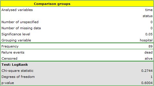
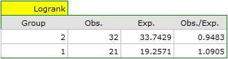

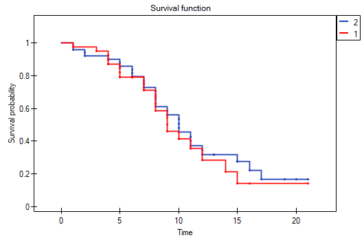
On the basis of the significance level  , based on the obtained value p=0.6004 for the log-rank test (p=0.6959 for Gehan's and 0.6465 for Tarone-Ware) we conclude that there is no basis for rejecting the hypothesis
  . The length of life calculated for the patients of both hospitals is similar.
The same conclusion will be reached when comparing the risk of death for those hospitals by determining the risk ratio. The obtained estimated value is HR=1.1499 and 95% of the confidence interval for that value contains 1:  0.6570, 2.0126
 .
.
Differences for many survival curves
Liver transplantations were made for people at different ages. 3 age groups were distinguished:  years
years years
years </latex>,
  years
years years
years ,
,  years
years years. We will check if the patients' survival time after transplantations depended on their age at the time of the transplantation.
Hypotheses:

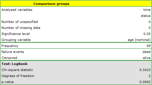
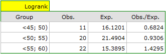
On the basis of the significance level , based on the obtained value p=0.0692 in the log-rank test (p=0.0928 for Gehan's and p=0.0779 for Tarone-Ware) we conclude that there is no basis for the rejection of the hypothesis . The length of life calculated for the patients in the three compared age groups is similar. However, it is noticeable that the values are quite near to the standard significance level 0.05.
When examining the hazard values (the ratio of the observed values and the expected failure events) we notice that they are a little higher with each age group (0.68, 0.93, 1.43). Although no statistically significant differences among them are seen it is possible that a growth trend of the hazard value (trend in the position of the survival rates) will be found.
Trend for many survival curves
If we introduce into the test the information about the ordering of the compared categories (we will use the age variable in which the age ranges will be numbered, respectively, 1, 2, and 3), we will be able to check if there is a trend in the compared curves. We will study the following hypotheses:


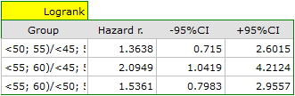
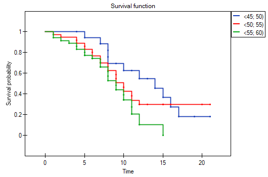
On the basis of the significance level , based on the obtained value p=0.0237 in the log-rank test (p=0.0317 for Gehan's and p=0.0241 for Tarone-Ware) we conclude that the survival curves are positioned in a certain trend. On the Kaplan-Meier graph the curve for people aged  </latex>55 years; 60 years) is the lowest. Above that curve there is the curve for patients aged 50 years; 55 years). The highest curve is the one for patients aged 45 years; 50 years). Thus, the older the patient at the time of a transplantation, the lower the probability of survival over a certain period of time.
Survival curves for stratas
Let us now check if the trend observed before is independent of the hospital in which the transplantation took place. For that purpose we will choose a hospital as the stratum variable.
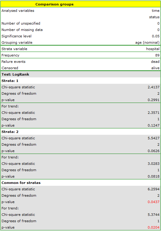
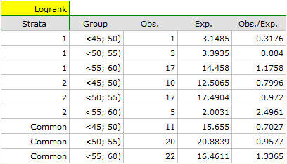
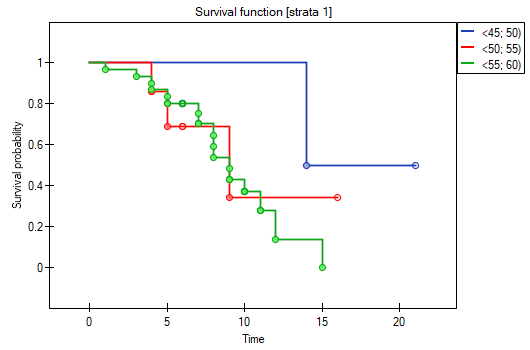
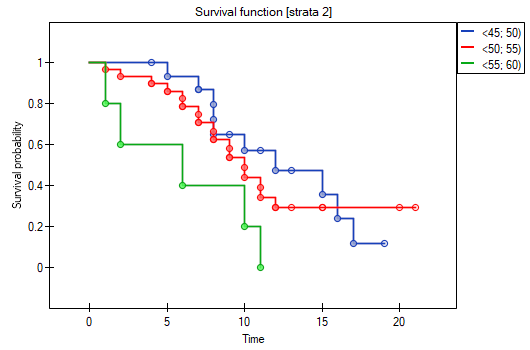
The report contains, firstly, an analysis of the strata: both the test results and the hazard ratio. In the first stratum the growing trend of hazard is visible but not significant. In the second stratum a trend with the same direction (a result bordering on statistical significance) is observed. A cumulation of those trends in a common analysis of strata allowed the obtainment of the significance of the trend of the survival curves. Thus, the older the patient at the time of a transplantation, the lower the probability of survival over a certain period of time, independently from the hospital in which the transplantation took place.
A comparative analysis of the survival curves, corrected by strata, yields a result significant for the log-rank and Tarone-Ware tests and not significant for Gehan's test, which might mean that the differences among the curves are not so visible in the initial survival periods as in the later ones. By looking at the hazard ratio of the curves compared in pairs
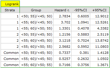
we can localize significant differences. For the comparison of the curve of the youngest group with the curve of the oldest group the hazard ratio is the smallest, 0.53, the 95\% confidence interval for that ratio, 0.26 ; 1.05, does contain value 1 but is on the verge of that value, which can suggest that there are significant differences between the respective curves. In order to confirm that supposition an inquisitive researcher can, with the use of the data filter in the analysis window, compare the curves in pairs.
However, it ought to be remembered that one of the corrections for multiple comparisons should be used and the significance level should be modified. In this case, for Bonferroni's correction, with three comparisons, the significance level will be 0.017. For simplicity, we will only avail ourselves of the log-rank test.
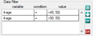
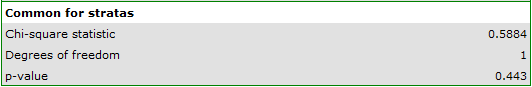
45 lat; 50 lat) vs 50 lat; 55 lat)
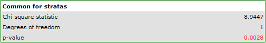
45 lat; 50 lat) vs 55 lat; 60 lat)
50 lat; 55 lat) vs 55 lat; 60 lat)
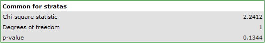
As expected, statistically significant differences only concern the survival curves of the youngest and oldest groups.
en/statpqpl/survpl/kmporpl/warstwpl.txt · ostatnio zmienione: 2022/02/16 10:03 przez admin
Narzędzia strony
Wszystkie treści w tym wiki, którym nie przyporządkowano licencji, podlegają licencji: CC Attribution-Noncommercial-Share Alike 4.0 International
