PQStat - Baza Wiedzy

Example for multiple regression

EXAMPLE (publisher.pqs file)

A certain book publisher wanted to learn how was gross profit from sales influenced by such variables as: production cost, advertising costs, direct promotion cost, the sum of discounts made, and the author's popularity. For that purpose he analyzed 40 titles published during the previous year (teaching set). A part of the data is presented in the image below:

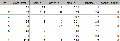
The first five variables are expressed in thousands fo dollars - so they are variables gathered on an interval scale. The last variable: the author's popularity – is a dychotomic variable, where 1 stands for a known author, and 0 stands for an unknown author.

On the basis of the knowledge gained from the analysis the publisher wants to predict the gross profit from the next published book written by a known author. The expenses the publisher will bear are: production cost $\approx 11$ , advertising costs $\approx 13$ , direct promotion costs $\approx 0.5$ , the sum of discounts made $\approx 0.5$ .

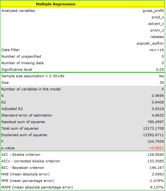
We construct the model of multiple linear regression, for teaching dataset, selecting: gross profit – as the dependent variable $Y$ , production cost, advertising costs, direct promotion costs, the sum of discounts made, the author's popularity – as the independent variables $X_1, X_2, X_3, X_4, X_5$ . As a result, the coefficients of the regression equation will be estimated, together with measures which will allow the evaluation of the quality of the model.

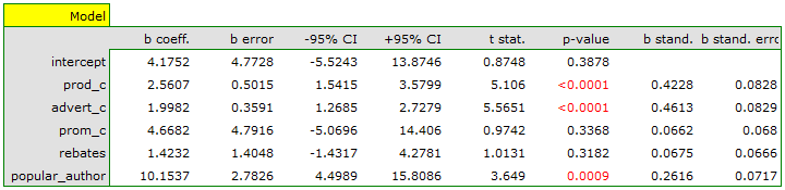
On the basis of the estimated value of the coefficient $b$ , the relationship between gross profit and all independent variables can be described by means of the equation: $\begin{displaymath} profit_{gross}=4.18+2.56(c_{prod})+2(c_{adv})+4.67(c_{prom})+1.42(discounts)+10.15(popul_{author})+[8.09] \end{displaymath}$ The obtained coefficients are interpreted in the following manner:

If the production cost increases by 1 thousand dollars, then gross profit will increase by about 2.56 thousand dollars, assuming that the remaining variables do not change;
If the production cost increases by 1 thousand dollars, then gross profit will increase by about 2 thousand dollars, assuming that the remaining variables do not change;
If the production cost increases by 1 thousand dollars, then gross profit will increase by about 4.67 thousand dollars, assuming that the remaining variables do not change;
If the sum of the discounts made increases by 1 thousand dollars, then gross profit will increase by about 1.42 thousand dollars, assuming that the remaining variables do not change;
If the book has been written by a known author (marked as 1), then in the model the author's popularity is assumed to be the value 1 and we get the equation:

$\begin{displaymath} profit_{gross}=14.33+2.56(c_{prod})+2(c_{adv})+4.67(c_{prom})+1.42(discounts) \end{displaymath}$

If the book has been written by an unknown author (marked as 0), then in the model the author's popularity is assumed to be the value 0 and we get the equation: $\begin{displaymath} profit_{gross}=4.18+2.56(c_{prod})+2(c_{adv})+4.67(c_{prom})+1.42(discounts) \end{displaymath}$

The result of t-test for each variable shows that only the production cost, advertising costs, and author's popularity have a significant influence on the profit gained. At the same time, that standardized coefficients $b$ are the greatest for those variables.

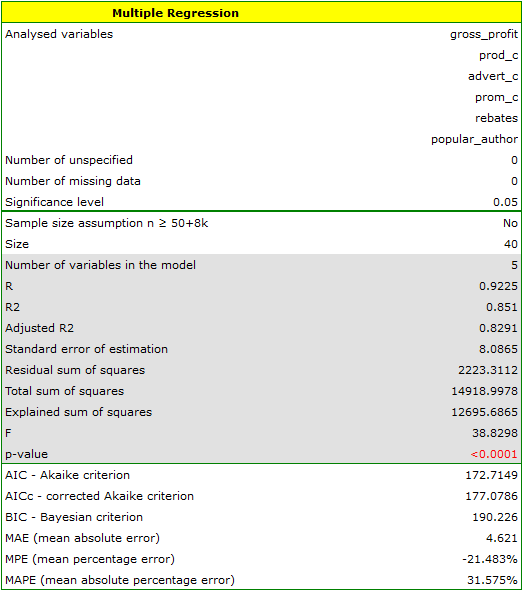
Additionally, the model is very well-fitting, which is confirmed by: the small standard error of estimation $SE_e=8.087$ , the high value of the multiple determination coefficient $R^2=0.85$ , the corrected multiple determination coefficient $R_{adj}^2= 0.83$ , and the result of the F-test of variance analysis: p<0.0001.

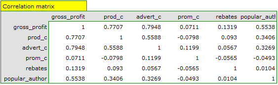
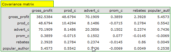
On the basis of the interpretation of the results obtained so far we can assume that a part of the variables does not have a significant effect on the profit and can be redundant. For the model to be well formulated the interval independent variables ought to be strongly correlated with the dependent variable and be relatively weakly correlated with one another. That can be checked by computing the correlation matrix and the covariance matrix:

The most coherent information which allows finding those variables in the model which are redundant is given by the parial and semipartial correlation analysis as well as redundancy analysis:

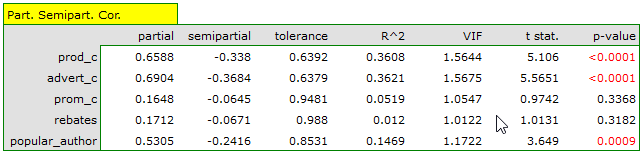
The values of coefficients of partial and semipartial correlation indicate that the smallest contribution into the constructed model is that of direct promotion costs and the sum of discounts made. However, those variables are the least correlated with model residuals, which is indicated by the low value $R^2$ and the high tolerance value. All in all, from the statistical point of view, models without those variables would not be worse than the current model (see the result of t-test for model comparison). The decision about whether or not to leave that model or to construct a new one without the direct promotion costs and the sum of discounts made, belongs to the researcher. We will leave the current model.

Finally, we will analyze the residuals. A part of that analysis is presented below:

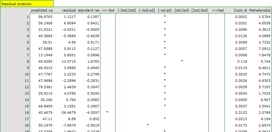
It is noticeable that one of the model residuals is an outlier – it deviates by more than 3 standard deviations from the mean value. It is observation number 16. The observation can be easily found by drawing a chart of residuals with respect to observed or expected values of the variable $Y$ .

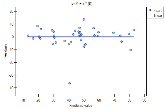
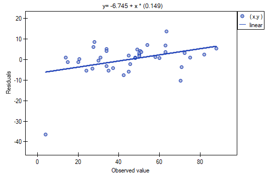
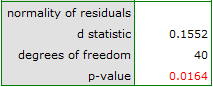
That outlier undermines the assumption concerning homoscedasticity. The assumption of homoscedasticity would be confirmed (that is, residuals variance presented on the axis $Y$ would be similar when we move along the axis $X$ ), if we rejected that point. Additionally, the distribution of residuals deviates slightly from normal distribution (the value $p$ of Liliefors test is p=0.0164):

When we take a closer look of the outlier (position 16 in the data for the task) we see that the book is the only one for which the costs are higher than gross profit (gross profit=4 thousand dollars, the sum of costs = (8+6+0.33+1.6) = 15.93 thousand dollars).

The obtained model can be corrected by removing the outlier. For that purpose, another analysis has to be conducted, with a filter switched on which will exclude the outlier.

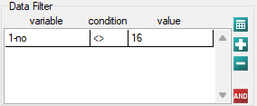
As a result, we receive a model which is very similar to the previous one but is encumbered with a smaller error and is more adequate:

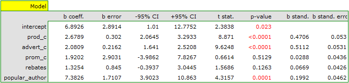
$\begin{displaymath} profit_{gross}=6.89+2.68(c_{prod})+2.08(c_{adv})+1.92(c_{prom})+1.33(discounts)+7.38(popul_{author})+[4.86] \end{displaymath}$

The final version of the model will be used for prediction. On the basis of the predicted costs amounting to: production cost $\approx 11$ thousand dollars,\\advertising costs $\approx 13$ thousand dollars,\\direct promotion costs $\approx 0.5$ thousand dollars,\\the sum of discounts made $\approx 0.5$ thousand dollars,\\and the fact that the author is known (the author's popularity $\approx 1$ ) we calculate the predicted gross profit together with the confidence interval:

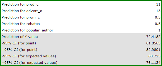
The predicted profit is 72 thousand dollars.

Finally, it should still be noted that this is only a preliminary model. In a proper study more data would have to be collected. The number of variables in the model is too small in relation to the number of books evaluated, i.e. n<50+8k.

PQStat - Baza Wiedzy

Narzędzia użytkownika

Narzędzia witryny

Pasek boczny

Example for multiple regression

Narzędzia strony