PQStat - Baza Wiedzy

Introduction

The most familiar image associated with meta-analysis is the forest plot showing the results of each study along with a summary.

$\begin{pspicture}(-2,-0.5)(5,4) \psline{-}(1.4,0)(1.4,4) \psline{->}(0,0)(5,0) \psline[linewidth=0.7pt, linestyle=dotted](2.6,0)(2.6,4) \rput(-0.8,0.8){\scriptsize Summary} \psdiamond[framearc=.3,fillstyle=solid, fillcolor=lightgray](2.6,0.8)(0.4,0.15) \rput(-0.6,1.575){\scriptsize Study 5} \psline[linewidth=0.2pt](2.3,1.575)(2.9,1.575) \psframe[linewidth=0.1pt,framearc=.1,fillstyle=solid, fillcolor=lightgray](2.5,1.5)(2.65,1.65) \rput(-0.6,2.1){\scriptsize Study 4} \psline[linewidth=0.2pt](2.53,2.1)(3.1,2.1) \psframe[linewidth=0.1pt,framearc=.1,fillstyle=solid, fillcolor=lightgray](2.7,2)(2.9,2.2) \rput(-0.6,2.54){\scriptsize Study 3} \psline[linewidth=0.2pt](1,2.54)(3.35,2.54) \psframe[linewidth=0.1pt,framearc=.1,fillstyle=solid, fillcolor=lightgray](2,2.5)(2.08,2.58) \rput(-0.6,3.04){\scriptsize Study 2} \psline[linewidth=0.2pt](1.25,3.04)(3.25,3.04) \psframe[linewidth=0.1pt,framearc=.1,fillstyle=solid, fillcolor=lightgray](2.1,3)(2.18,3.08) \rput(-0.6,3.55){\scriptsize Study 1} \psline[linewidth=0.2pt](0.85,3.55)(2.5,3.55) \psframe[linewidth=0.1pt,framearc=.1,fillstyle=solid, fillcolor=lightgray](1.5,3.5)(1.6,3.6) \rput(2.4,-0.3){\scriptsize Effect size} \end{pspicture}$

In order for the selected literature to be summarized together, it must be consistent in description and the measures given there must be the same.

To be used in a meta-analysis, a scientific paper should describe:

Final result which is some kind of statistical measure indicating the result (effect) obtained in the paper. In fact, these can be different kinds of measures, e.g., difference between means, odds ratio, relative risk, etc.

Standard Error i.e. SE allowing one to determine the precision of the study carried out. This precision assigns the study weight. The smaller the error (SE), the higher the precision of a given study and the higher the assigned weight will be, making a given study more likely to contribute to the results of a meta-analysis.

Group size is the number of objects on which the study was conducted.

Note

It often happens, that a scientific paper does not contain all of the elements listed above, in which case you should look for data in the paper from which the calculation of these measures will be possible.

Note

The PQstat program performs meta-analysis related calculations on data containing: Final Effect, Standard Error, and in some situations Group Size. It is recommended that you enter the data for each publication in the data preparation window before performing the meta-analysis. This is particularly handy when a paper does not explicitly provide these three measures.

The data preparation window is opened via menu: Advanced Statistics→Meta-analysis→Data preparation.

In the data preparation window for meta-analysis, the researcher first provides the name of the study being entered. This name should uniquely identify the study, as it will describe it in all meta-analysis results, including graphs. The desired Final result, Effect Error and Group Size are calculated based on measures extracted from the relevant scientific paper. The measures included in the studies from which the final results can be calculated are shown in the table below:

$\begin{tabular}{|c|c|c|} \hline Study type&Study measures&Final result\\\hline\hline Independent means&Means, st. deviations&\textbf{a}, \textbf{b}, \textbf{c}, \textbf{e}\\ &Means, SE&\textbf{a}, \textbf{b}, \textbf{c}, \textbf{e}\\ &Difference, interval&\textbf{a}\\ &d Cohen, interval&\textbf{b}\\ &g Hadges, interval&\textbf{c}\\ &Ratio, interval&\textbf{e}\\ &Difference, SE&\textbf{a}\\ &d Cohen, SE&\textbf{b}\\ &g Hadges, SE&\textbf{c}\\ &Ratio, SE&e\\\hline Dependent means&Means, st. deviations&\textbf{a}, \textbf{b}, \textbf{c}\\ &Means, SE&\textbf{a}, \textbf{b}, \textbf{c}\\ &Difference, interval&\textbf{a}\\ &d Cohen, interval&\textbf{b}\\ &g Hadges, interval&\textbf{c}\\ &Difference, st. deviation&\textbf{a}, \textbf{b}, \textbf{c}\\ &Difference, SE&\textbf{a}, \textbf{b}, \textbf{c}\\ &d Cohen, SE&\textbf{b}\\ &g Hadges, SE&\textbf{c}\\\hline Mean vs. set&Mean, st. deviation&\textbf{a}\\ &Mean, SE&\textbf{a}\\\hline Mean - summary&Mean, st. deviation&\textbf{d}\\ &Mean, SE&\textbf{d}\\\hline Tables &2x2 Tables&\textbf{b}, \textbf{c}, \textbf{f}, \textbf{g}, \textbf{h}\\ &OR, interval&\textbf{b}, \textbf{c}, \textbf{f}\\ &RR, interval&\textbf{g}\\ &RD, interval&\textbf{h}\\ &d Cohen, interval&\textbf{b}, \textbf{c}, \textbf{f}\\ &g Hadges, interval&\textbf{b}, \textbf{c}, \textbf{f}\\ &OR, SE&\textbf{b}, \textbf{c}, \textbf{f}\\ &RR, SE&\textbf{g}\\ &RD, SE&\textbf{h}\\ &d Cohen, SE&\textbf{b}, \textbf{c}, \textbf{f}\\ &g Hadges, SE&\textbf{b}, \textbf{c}, \textbf{f}\\\hline Correlation&Coefficient&\textbf{i}\\ &Coefficient, interval&\textbf{i}\\ &Coefficient, SE&\textbf{i}\\\hline ROC curve&AUC, SE&\textbf{j}\\ &AUC, interval&\textbf{j}\\\hline One proportion&Set group size&\textbf{k}\\ &Set proportion&\textbf{k}\\\hline \end{tabular}$

where the individual end results are:

a – Difference of means
b – d Cohen
c – g Hadges
d – Mean
e – Ratio of means
f – Odds Ratio (OR)
g – Relative risk (RR)
h – Risk differential (RD)
i – Pearson coefficient
j – AUC (ROC curve)
k – Proportion

Note

In determining the error of coefficients such as OR or RR and others based on tables, when there exist values of zero in the tables or in determining the error of proportions when the proportion is 0 or 1, a continuity correction using an increase factor of 0.5 is applied. The confidence interval for proportions is determined according to the exact Clopper-Pearson method\cite{clopper_pearson}.

EXAMPLE

We are interested in the effect of cigarette smoking on the risk of disease X. We want to conduct a meta-analysis for which the end result will be relative risk (RR). Under this assumption, the papers selected for the meta-analysis must be able to calculate the RR and its error.

Step 1. Based on the description of the final result (see table above), it was found that the relative risk (described as the score g) is possible to determine in the PQStat program in three situations, i.e., if the RR and the confidence interval for it or the RR together with the error are given in the scientific paper, or if the corresponding group sizes in four categories are given, i.e., a 2×2 table.

Step 2. Ten papers were selected for meta-analysis that met the inclusion criteria and had the potential to determine relative risk (see step 1). The needed data included in the selected papers were:

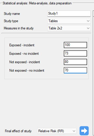
Study 1: group sizes: (smokers and sick)=100, (smokers and non-sick)=73, (non-smokers and sick)=80, (non-smokers and non-sick)=70,

Study 2: group sizes: (smokers and sick)=182, (smokers and non-sick)=172, (non-smokers and sick)=180, (non-smokers and non-sick)=172,

Study 3: group sizes: (smokers and sick)=157, (smokers and non-sick)=132, (non-smokers and sick)=125, (non-smokers and non-sick)=201,

Study 4: group sizes: (smokers and sick)=19, (smokers and non-sick)=15, (non-smokers and sick)=35, (non-smokers and non-sick)=20,

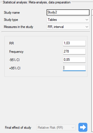
Study 5: group size: 278, RR[95\%CI]=1.03[0.85-1.25],

Study 6: group size: 560, RR[95\%CI]=1.21[1.05-1.40],

Study 7: group size: 1207, RR[95\%CI]=1.04[0.93-1.15],

Study 8: group size: 214, RR[95\%CI]=1.15[0.95-1.40],

Study 9: group size: 285, RR[95\%CI]=1.36[1.03-1.79],

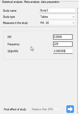
Study 10: group size: 1968, RR=1.17, SE(lnRR)=0.0437,

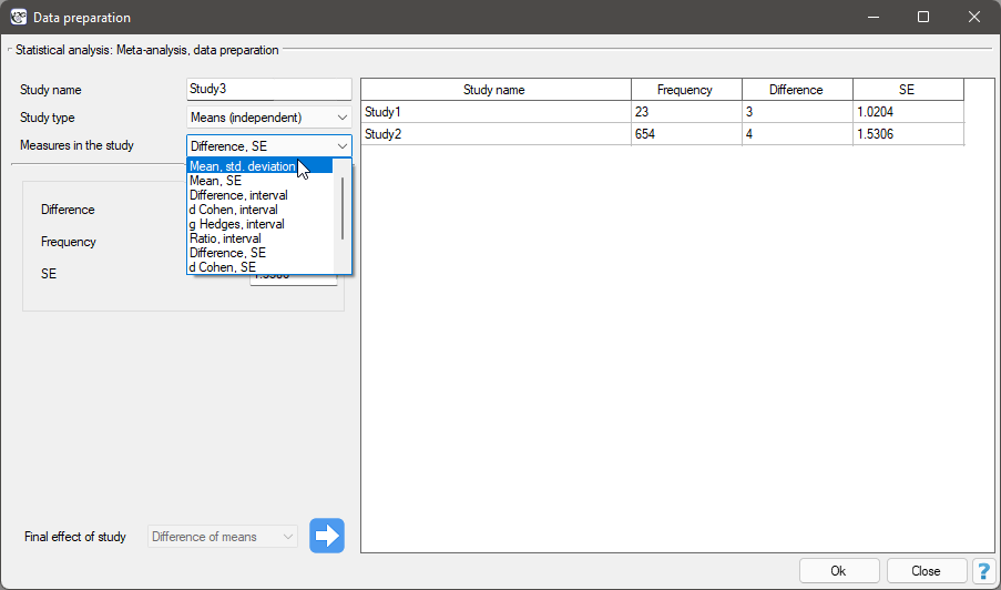
Step 3. KUsing the study preparation window for the meta-analysis, data was input into the datasheet. The first four studies are entered by selecting tables, studies five through nine are entered by selecting RR and range, and the last study provides all the necessary data, i.e., RR and SE. We set Relative risk (RR) as the Final effect of the study:

We move each entered study to the window on the right-hand side . Using the OK button, we transfer the prepared studies to the datasheet. Based on the information about each study in the datasheet, you can proceed to perform a meta-analysis.

P-value, and thus statistical significance is not directly used in meta-analysis. The same effect size may be statistically significant in a large study and insignificant in a study based on small sample size. Moreover, a quite small effect size may be statistically significant in a large study, and a quite large effect size may be insignificant in a small study. This fact is related to the power of statistical tests. When testing for statistical significance, we are testing whether an effect exists at all, i.e., whether it is different from zero, not whether it is large enough to translate into desired effects. For example, the fact that a drug statistically significantly lowers blood pressure by 1mmHg will not result in it being used, because 1mmHg is too small from a clinical perspective. Meta-analysis focuses on the magnitude of individual effects rather than their statistical significance. As a result, it does not matter much whether the papers used in the meta-analysis indicate statistical significance of a particular effect or not.

In PQStat, statistical significance is calculated for each study given the effect ratio and the error of that effect. This is an asymptotic approach, based on a normal distribution and dedicated to large samples. If a different test was used to check statistical significance in the cited study, the results obtained may differ slightly.

PQStat - Baza Wiedzy

Narzędzia użytkownika

Narzędzia witryny

Pasek boczny

Introduction

Narzędzia strony