PQStat - Baza Wiedzy

Selection of optimum cut-off

The point which is looked for is a certain value of the diagnostic variable, which provides the optimum separation of the studied population into to groups: (+) in which the given phenomenon occurs and (–) in which the given phenomenon does not occur. The selection of the optimum cut-off is not easy because it requires specialist knowledge about the topic of the study. For example, different cut-offs will be required in, on the one hand, a test used for screening of a large group of people, e.g. for a mammography study, and, on the other hand, in invasive studies conducted for the purpose of confirming an earlier suspicion, e.g. in histopathology. With the help of an advanced mathematical apparatus we can find a cut-off which will be the most useful from the perspective of mathematics.

PQStat allows you to select the optimal cut-off point by:

Tangent method (cost index) – calculated based on sensitivity, specificity, cost of erroneous decisions and prevalence.

Errors which can be made when classifying the studied objects as belonging to group (+) and group (–) are false positive results ( $FP$ ) and false negative results ( $FN$ ). If committing those errors is equally costly (ethical, financial, and other costs), then in the field Cost FP and in the field Cost FN we enter the same positive value – usually 1. However, if we come to the conclusion that one type of error is encumbered with a greater cost than the other one, then we will assign appropriately greater weight to it.

The optimum cut-off value is calculated on the basis of sensitivity, specificity, and with the help of value $m$ – slope of the tangent line to the ROC curve. The slope angle $m$ is defined in relation to two values: the costs of wrong decisions and the prevalence coefficient. Normally the costs of wrong decisions have the value 1 and the prevalence coefficient is estimated from the sample. Knowing, a priori, the prevalence coefficient ( $P_{a priori}$ ) and the costs of wrong decisions, the user can influence the value $m$ and, consequently, the search for an optimum cut-off. As a result, the optimum cut-off is determined to be such a value of the diagnostic variable for which the formula:

$\begin{displaymath}\textrm{Sensitivity} - m\cdot(1- \textrm{Specificity})\end{displaymath}$

reaches the minimum (Zweig M.H. 1993¹⁾).

The optimum cut-off point of the diagnostic variable, selected as described above, will finally be marked on the ROC curve.

Costs graph – presents the calculated values of an wrong diagnosis together with their costs. The values are computed according to the formula:

$\begin{displaymath} cost=cost_{FP}\cdot FP+cost_{FN}\cdot FN \end{displaymath}$

The point marked on the graph is the minimum of the function presented above.

Youden's Index – Conceptually, it is the maximum distance between the line that is the diagonal of a square of side 1 and the point of the ROC curve ²⁾. This index is calculated from the formula:

$\begin{displaymath}d=\textrm{Sensitivity}+ \textrm{Specificity} -1\end{displaymath}$

The optimal cut-off point of the diagnostic variable thus selected will eventually be marked on the ROC curve plot.

Distance from the top left corner – Conceptually, it is the minimum distance between the upper left corner of a square of side 1 (i.e., the place where sensitivity and specificity can be highest) and the point of the ROC curve. This index is calculated from the formula:

$\begin{displaymath}d=\sqrt{(1-\textrm{Sensitivity})^2+(1-\textrm{Specificity})^2}\end{displaymath}$

The optimal cut-off point of the diagnostic variable thus selected will eventually be marked on the ROC curve plot.

Costs graph – presents the calculated values of an wrong diagnosis together with their costs. The values are computed according to the formula:

$\begin{displaymath} cost=cost_{FP}\cdot FP+cost_{FN}\cdot FN \end{displaymath}$

The point marked on the graph is the minimum of the function presented above.

Sensitivity and specificity intersection graph – allows the localization of the point in which the value of sensitivity and specificity is simultaneously the greatest.

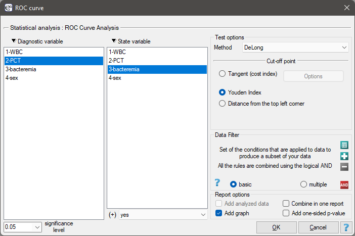
The window with settings for ROC analysis is accessed via the menu Advanced statistics → Diagnostic tests→ROC curve.

EXAMPLE (file bacteriemia.pqs)

Persistent high fever in an infant or a small child without clearly diagnosed reasons is a premise for testing for bacteremia. The most useful and reliable parameters for screening and monitoring bacterial infections are the following indicators:

WBC – the number of white blood cells
PCT – procalcitonin.

It is assumed that in a healthy infant or a small child WBC should not exceed 15 thousand/ $\mu$ and PCT should be lower than 0.5 ng/ml.

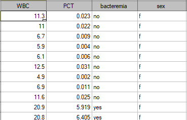
The sample values of those indicators for 136 children of up to 3 years old with persistent fever $>39^0C$ is presented in the table fragment below:

One method of analyzing the PCT indicator is transforming it into a dichotomous variable by selecting a cut-off (e.g. $x_{cat}$ =0.5 ng/ml) above which the study is considered to be „positive”. The level of adequacy of such a division will be indicated by the value of sensitivity and specificity. We want to use a more complex approach, that is, calculate the sensitivity and specificity not only for one value but for each PCT value obtained in the sample - which means constructing a ROC curve. On the basis of the information obtained in that manner we want to check if the PTC indicator is indeed useful for diagnosing bacteremia. If so, then we want to check what is the optimal cut-off above which we can consider the study to be „positive” – detecting bacteremia.

In order to check if PTC is really useful for diagnosing bacteremia we will calculate the size of the area under the ROC curve and verify the hypothesis that:

$\begin{array}{cl} \mathcal{H}_0: & $area under the constructed ROC curve $=0.5, \\ \mathcal{H}_1: & $area under the constructed ROC curve $\neq 0.5. \end{array}$

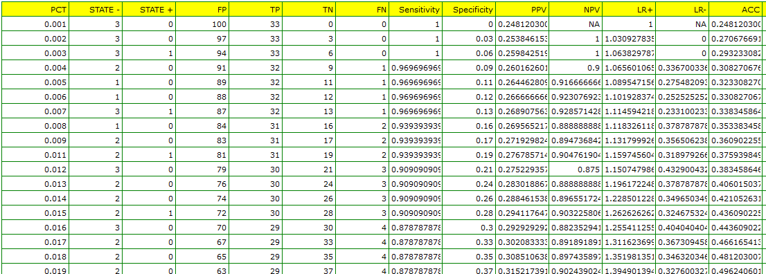
As bacteremia is accompanied by an increased PCT level, in the test options window we will consider the indicator to be a stimulant. In the state variable we have to define which value in the bacteremia column determines its presence, then we select „yes”. Apart from the result of the statistical test, in the report we can find an exact description of every possible cut-off.

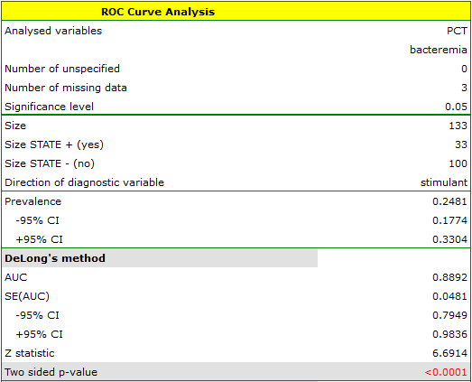
The calculated size of the area under the ROC curve is AUC=0.889. Therefore, on the basis of the adopted level $\alpha=0.05$ , based on the obtained value p<0.0001 we assume that diagnosing bacteremia with the use of the PCT indicator is indeed more useful than a random distribution of patients into 2 groups: suffering from bacteremia and not suffering from it. Therefore, we return to the analysis (button ) to define the optimal cut-off.

The algorithm of searching for the optimal cut-off takes into account the costs of wrong decisions and the prevalence coefficient.

FN cost - wrong diagnosis is the cost of assuming that the patient does not suffer from bacteremia although in reality he or she is suffering from it (costs of a falsely negative decision)
FP cost - wrong diagnosis, is the cost of assuming that the patient suffers from bacteremia although in reality he or she is not suffering from it (costs of a falsely positive decision)

As the FN costs are much more serious than the FP costs, we enter a greater value in field one than in field two. We decided the value would be 5.

The PCT value is to be used in screening so we do not give the prevalence coefficient for the population (a priori prevalence coefficient) which is very low but we use the estimated coefficient from the sample. We do so in order not to move the cut-off of the PCT value too high and not to increase the number of falsely negative results.

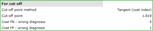
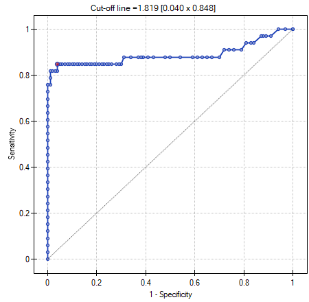
The optimal PCT cut-off determined in this way is 1.819. For this point sensitivity=0.85 and specificity=0.96.

Another method of selecting the cut-off is the anlysis of the costs graph and of the sensitivity intersection graph:

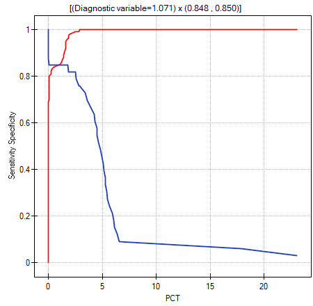
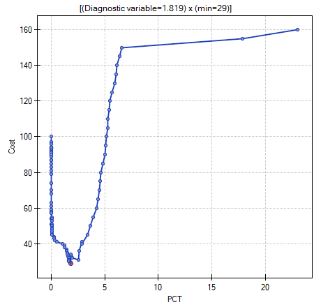
The analysis of the costs graph shows that the minimum of the costs of wrong decisions lies at PCT=1.819. The value of sensitivity and specificity is similar at PCT=1.071.

¹⁾

Zweig M.H., Campbell G. (1993), Receiver-operating characteristic (ROC) plots: a fundamental evaluation tool in clinical medicine. Clinical Chemistry 39:561-577

²⁾

Youden W.J. (1950), Index for rating diagnostic tests. Cancer. 3: 32–35

PQStat - Baza Wiedzy

Narzędzia użytkownika

Narzędzia witryny

Pasek boczny

Selection of optimum cut-off

Narzędzia strony