Contingency tables coefficients and their statistical significance
The contingency coefficients are calculated for the raw data or the data gathered in a contingency table.
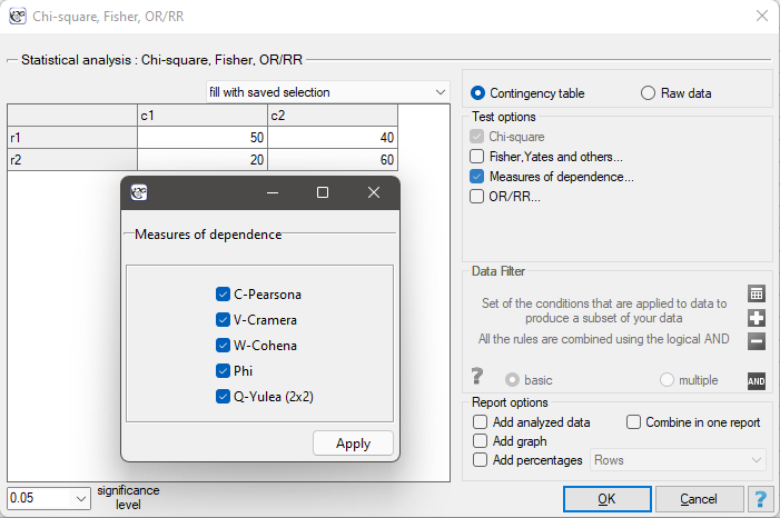
The settings window with the measures of correlation can be opened in Statistics menu → NonParametric tests → Ch-square, Fisher, OR/RR option Measures of dependence… or in ''Wizard''.
The Yule's Q contingency coefficient
The Yule's  contingency coefficient (Yule, 19001)) is a measure of correlation, which can be calculated for
  contingency tables.

where:
 - observed frequencies in a contingency table.
The coefficient value is included in a range of  . The closer to 0 the value of the is, the weaker dependence joins the analysed features, and the closer to
  1 or +1, the stronger dependence joins the analysed features. There is one disadvantage of this coefficient. It is not much resistant to small observed frequencies (if one of them is 0, the coefficient might wrongly indicate the total dependence of features).
The statistic significance of the Yule's coefficient is defined by the  test.
test.
Hypotheses:

The test statistic is defined by:

The test statistic asymptotically (for a large sample size) has the normal distribution.
The p-value, designated on the basis of the test statistic, is compared with the significance level  :
:

The Phi contingency coefficient is a measure of correlation, which can be calculated for contingency tables.

The  coefficient value is included in a range of
  . The closer to 0 the value of is, the weaker dependence joins the analysed features, and the closer to 1, the stronger dependence joins the analysed features.
The contingency coefficient is considered as statistically significant, if the p-value calculated on the basis of the  test (designated for this table) is equal to or less than the significance level .
The Cramer's V contingency coefficient
The Cramer's V contingency coefficient (Cramer, 19462)), is an extension of the coefficient on  contingency tables.

where:
Chi-square – value of the test statistic,
 – total frequency in a contingency table,
 – the smaller the value out of
  and
and  .
.
The  coefficient value is included in a range of . The closer to 0 the value of is, the weaker dependence joins the analysed features, and the closer to 1, the stronger dependence joins the analysed features. The coefficient value depends also on the table size, so you should not use this coefficient to compare different sizes of contingency tables.
The contingency coefficient is considered as statistically significant, if the p-value calculated on the basis of the test (designated for this table) is equal to or less than the significance level .
W-Cohen contingency coefficient
The  -Cohen contingency coefficient (Cohen (1988)3)), is a modification of the V-Cramer coefficient and is computable for tables.

where:
Chi-square – value of the test statistic,
– total frequency in a contingency table,
– the smaller the value out of and .
The coefficient value is included in a range of  , where
  (for tables where at least one variable contains only two categories, the value of the coefficient is in the range ). The closer to 0 the value of is, the weaker dependence joins the analysed features, and the closer to
  , the stronger dependence joins the analysed features. The coefficient value depends also on the table size, so you should not use this coefficient to compare different sizes of contingency tables.
The contingency coefficient is considered as statistically significant, if the p-value calculated on the basis of the test (designated for this table) is equal to or less than the significance level .
The Pearson's C contingency coefficient
The Pearson's  contingency coefficient is a measure of correlation, which can be calculated for contingency tables.

The coefficient value is included in a range of  . The closer to 0 the value of is, the weaker dependence joins the analysed features, and the farther from 0, the stronger dependence joins the analysed features. The coefficient value depends also on the table size (the bigger table, the closer to 1 value can be), that is why it should be calculated the top limit, which the coefficient may gain – for the particular table size:

where:
– the smaller value out of and .
An uncomfortable consequence of dependence of value on a table size is the lack of possibility of comparison the coefficient value calculated for the various sizes of contingency tables. A little bit better measure is a contingency coefficient adjusted for the table size ( ):
):

The contingency coefficient is considered as statistically significant, if the p-value calculated on the basis of the test (designated for this table) is equal to or less than significance level .
EXAMPLE (sex-exam.pqs file)
There is a sample of 170 persons ( ), who have 2 features analysed (
 =sex,
=sex,  =passing the exam). Each of these features occurs in 2 categories (
 =f,
=f,  =m,
=m,  =yes,
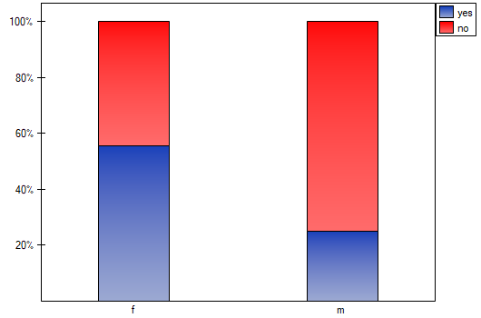
=yes,  =no). Basing on the sample, we would like to get to know, if there is any dependence between sex and passing the exam in an analysed population. The data distribution is presented in a contingency table:}

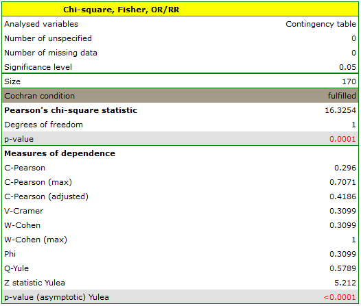
The test statistic value is  and the
  value calculated for it: p<0.0001. The result indicates that there is a statistically significant dependence between sex and passing the exam in the analysed population.
Coefficient values, which are based on the test, so the strength of the correlation between analysed features are:
-Pearson = 0.42.
-Cramer = = -Cohen = 0.31
The -Yule = 0.58, and the value of the test (similarly to test) indicates the statistically significant dependence between the analysed features.