ANCOVA
Analysis of covariance (ANCOVA) is a method of testing the hypothesis that the means of two or more populations are equal, in correction for other continuous variables. These adjustments result in effects more readily seen by researchers than those obtained through ANOVA, i.e., narrower confidence intervals and greater statistical power.
Suppose an experiment is conducted to evaluate the effects of two treatments. The groups randomly assigned to treatment differ slightly in mean age, which also affects the treatment effect. Differences between groups in achievement will be quite ambiguous to interpret, since the groups differ in both age and treatment conditions. Analysis of covariance will provide „adjusted averages”, which estimate what the mean scores would be if the groups were exactly the same in terms of age. At the same time, the within-group variability of the results due to the variable (age) will be removed from the error variability to increase the precision of the test of the differences between the adjusted averages.
The label „analysis of covariance” is now seen as anachronistic by some research methodologists and statisticians, since this analysis is not a separate analysis but a variant of the general linear model (GLM). However, the term is still useful because it immediately conveys to most researchers the notion that a categorical variable (e.g., treatment conditions) and a continuous variable (e.g., age) are involved in a single analysis that determines treatment outcome.
The settings window with the ANCOVA can be opened in Advanced statistics→Multivariate models→ANCOVA
Note!!!
How to take into account the study factors and confounding variables is described in the section on multivariate ANOVA (Influence of confounding factors). The recommended way is to choose Sum of Squares type III and effects coding.
Basic application conditions:
- measurement on an interval scale,
- the samples come from a population with a normal distribution (normality of the variables or residuals of the model),
- equality of variances of an analysed variable in all populations,
- Equality of the slopes of the regression lines (regression coefficients between each confounding variable and the dependent variable) for each possible factor level.
Note!
Equality of the slopes of the regression lines is tested using the F test comparing the model containing the analyzed factors with the same model, but augmented by interactions with the confounding factors. A statistically significant result means that the assumption of equal slopes is violated, because the interaction becomes significant, so the different slopes of the simple.
ANCOVA hypotheses for a single factor  :
:

where:
 ,
, ,…,
,…, - expected averages of the factor for each of its categories.
ANCOVA hypotheses for factor interactions  :
:

where:
,,…, - expected average interactions of factors for their respective categories.
EXample(drug cholesterol.pqs file)
Imagine that a researcher was conducting a study on a new cholesterol-lowering drug. The study was designed so that the dose of the drug occurred at three levels: high, low and placebo. The researcher tested (using ANOVA independent) whether cholesterol after treatment differed according to the dose of the drug.
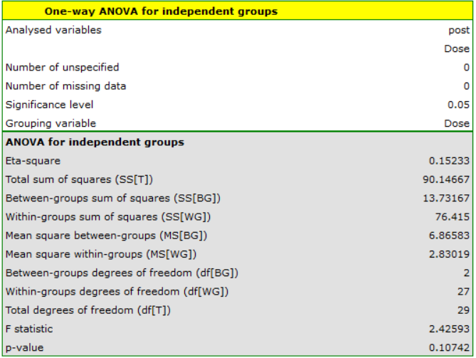
Unfortunately, the researcher did not get confirmation of the differences between the results.
Let's imagine that the researcher, realized that whether a drug would change cholesterol levels might be related to the patient's baseline cholesterol level and age. Therefore, he decided to perform a univariate ANCOVA (the factor is the dose of the drug) taking into account pre-treatment cholesterol levels and age as co-variables.
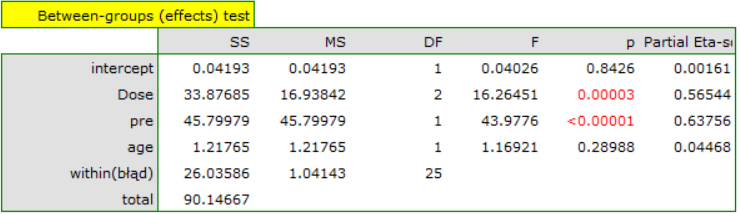
This time, the ANOCVA result indicated that there were significant differences between cholesterol levels after different doses of the drug (p=0.00003):
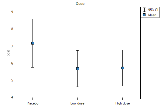
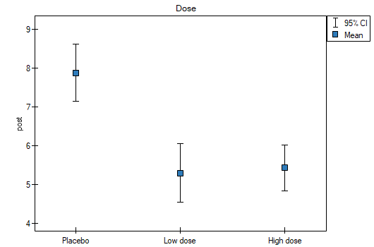
Including pre-test cholesterol levels reduced the obtained errors for the averages and narrowed the confidence intervals. To display the observed or expected averages, I choose the appropriate settings via Factor Options, to which I select the error graph. The first graph shows the observed averages with confidence interval, i.e., not including the effect of age and pre-treatment cholesterol levels; the second graph is the expected averages based on the built model with confidence intervals, i.e., after accounting for the effect of these two co-variables:
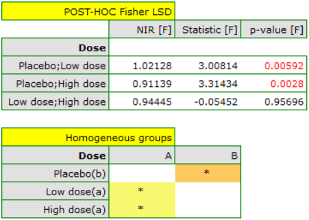
As a result, by taking into account the cholesterol level before treatment, the researcher was able to demonstrate the effectiveness of the new treatment. Cholesterol levels before treatment and age explain to some extent the changes in cholesterol levels after treatment, but we can attribute the rest of the changes in 57% to the drug dose used (partial Eta-square =0.565437). Post-hoc tests (selected by Factor options) suggested the formation of two homogeneous groups, the placebo group and the drug patient group, indicating that raising the dose to a high one does not make a difference, since the cholesterol levels obtained will be similar.
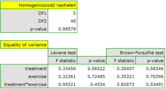
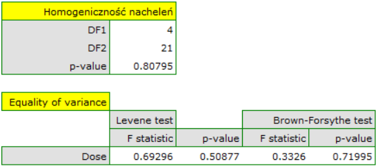
ANCOVA assumptions remained to be tested. Homogeneity of variance and constancy of slopes of simple regressions were confirmed using tests.
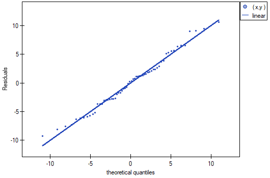
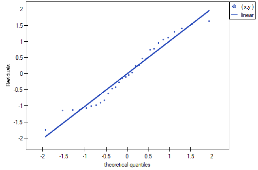
The normality of the rhesus distribution was assessed visually by plotting Q-Q plots:
The example comes from the Datarium R-Cran package.
Researchers want to evaluate the effect of a new treatment and exercise on stress reduction after accounting for differences in age. The value of the stress measure is the interval outcome variable Y. Because the variables „treatment” and „exercise” have 2 and 3 categories, respectively, we will conduct a two-way ANCOVA to determine whether the interaction between exercise and treatment, while accounting for the subjects' age, is related to stress.

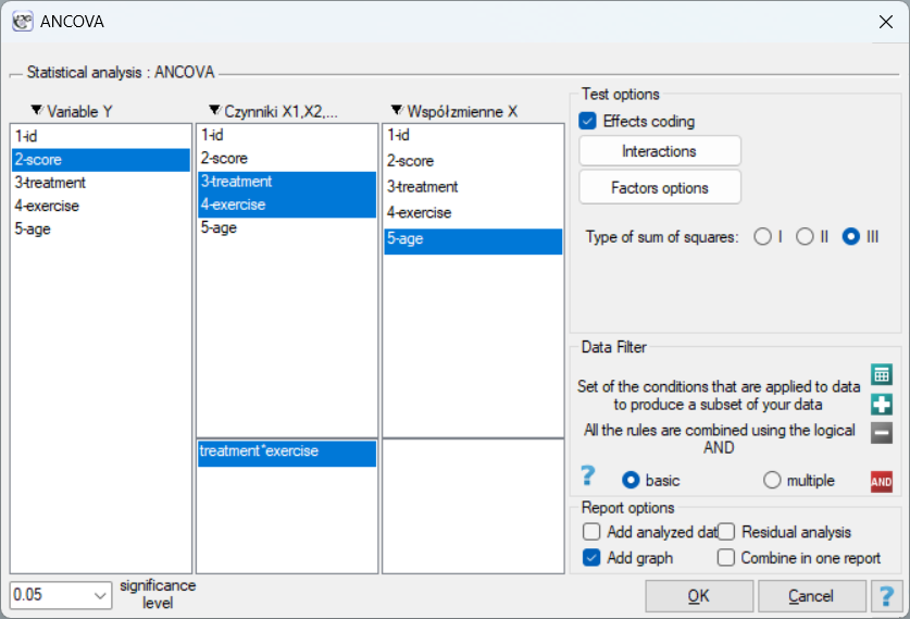
In the analysis window, I set „stress” as the dependent variable, „treatment” and „exercise” as factors, and add the interaction of these two variables, the continuous co-variable is „age.”
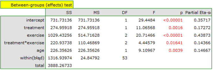
The result shows that the effect of treatment on stress varies with exercise intensity - indicated by a significant interaction of the two variables (p=0.016409). We plot a graph showing the expected mean stress levels for each of the six subgroups into which the interaction divided our data, and determine post-hoc tests.
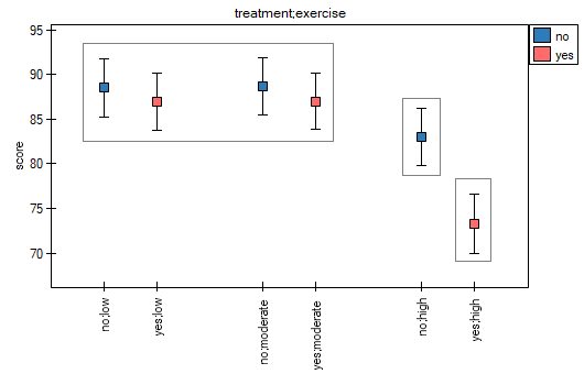
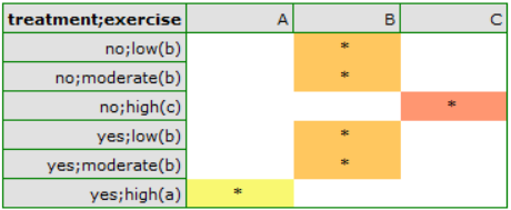
According to the results of the post-hoc test, we can speak of three different homogeneous groups: (B) the high-stress group is the group that exercises little or on average (whether or not they are treated sauropods), (C) the lower-stress group is the group that exercises a lot and is not treated, (A) the lowest-stress group is the group that exercises a lot and is treated. The values of the individual averages with confidence intervals are shown in the table
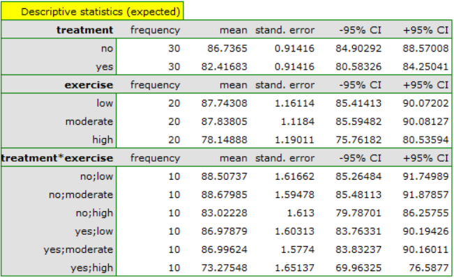
Assumptions regarding equality of variances, slopes of regression lines and normality of model residuals are met.